Page 37 - Process Modelling and Simulation With Finite Element Methods

24 Process Modelling and Simulation with Finite Element Methods

enough to do so is important information that will benefit the reader in later
chapters, where very clearly FEMLAB is the first choice package for the analysis
- 2-D and 3-D spatial-temporal systems with multiphysics.

1.2 Method 1: Root Finding

Typically, courses in numerical analysis go into great detail in the description of
the algorithm classes used for root finding, From experience, there are only two
algorithms that are really useful - the bisection method and Newton’s method.
Instead of presenting all the methods, here we will consider why root finding is
one of the most useful numerical analysis tools. Finding roots in linear systems
is fairly easy. Nonlinear systems are the challenge, and nearly all interesting
dynamics stem from nonlinear systems. The interest in root finding in nonlinear
systems results from its utility in describing inverse functions. Why? Because
with most nonlinear functions, the “forward direction”, y=f(u), is well described,
but the inverse function of u=f ‘(y) may be analytically indescribable, multi-
valued (non-unique), or even non-existent. But if it exists, then the numerical
description of an inverse function is identical to a root finding problem - find u
such that F(u)=O is equivalent to F(u)=f(u)-y=O. Since the goal of most analysis
is to find a solution of a set of constraints on a system, this is equivalent to
inverting the set of constraints. FEMLAB has a core function for solving
nonlinear systems, femnlin, and in this section its use to solve 0-D root finding
problems will be illustrated.
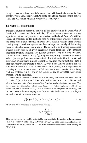
femnlin uses Newton’s method which with only one variable u uses the first
derivative F’(u) which is used iteratively to drive toward the root. The method
takes a local estimate of the slope of the function and projects to the root. The
slope can be computed either analytically (Newton-Raphson Method) or
numerically (the secant method). If the slope can be computed either way, you
can use Taylor’s theorem to project to the root. The basic idea is to use a Taylor
expansion about the current guess UO:

f (u) = f (uo ) + (. - uo ) f”uo ) + *.*

which can be re-arranged to estimate the root as

This methodology is readily extendable to a multiple dimension solution space,
i.e. u is a vector of unknowns, and division byf(u0) represents multiplication by
the inverse of the Jacobian off. The next subsection illustrates root finding in
FEMLAB .