Page 101 -

3.6 Quality of Resulting Models 83

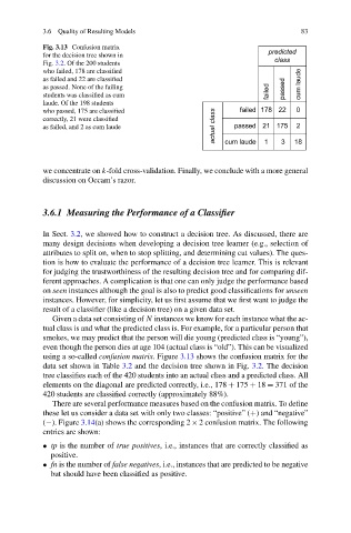
Fig. 3.13 Confusion matrix
for the decision tree shown in
Fig. 3.2. Of the 200 students
who failed, 178 are classified
as failed and 22 are classified
as passed. None of the failing
students was classified as cum
laude. Of the 198 students
who passed, 175 are classified
correctly, 21 were classified
as failed, and 2 as cum laude

we concentrate on k-fold cross-validation. Finally, we conclude with a more general
discussion on Occam’s razor.

3.6.1 Measuring the Performance of a Classifier

In Sect. 3.2, we showed how to construct a decision tree. As discussed, there are
many design decisions when developing a decision tree learner (e.g., selection of
attributes to split on, when to stop splitting, and determining cut values). The ques-
tion is how to evaluate the performance of a decision tree learner. This is relevant
for judging the trustworthiness of the resulting decision tree and for comparing dif-
ferent approaches. A complication is that one can only judge the performance based
on seen instances although the goal is also to predict good classifications for unseen
instances. However, for simplicity, let us first assume that we first want to judge the
result of a classifier (like a decision tree) on a given data set.
Given a data set consisting of N instances we know for each instance what the ac-
tual class is and what the predicted class is. For example, for a particular person that
smokes, we may predict that the person will die young (predicted class is “young”),
even though the person dies at age 104 (actual class is “old”). This can be visualized
using a so-called confusion matrix. Figure 3.13 shows the confusion matrix for the
data set shown in Table 3.2 and the decision tree shown in Fig. 3.2. The decision
tree classifies each of the 420 students into an actual class and a predicted class. All
elements on the diagonal are predicted correctly, i.e., 178 + 175 + 18 = 371 of the
420 students are classified correctly (approximately 88%).
There are several performance measures based on the confusion matrix. To define
these let us consider a data set with only two classes: “positive” (+) and “negative”
(−). Figure 3.14(a) shows the corresponding 2 × 2 confusion matrix. The following
entries are shown:
• tp is the number of true positives, i.e., instances that are correctly classified as
positive.
• fn is the number of false negatives, i.e., instances that are predicted to be negative
but should have been classified as positive.