Page 148 - Reliability and Maintainability of In service Pipelines

134 Reliability and Maintainability of In-Service Pipelines

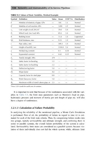
TABLE 5.5 Values of Basic Variables, Worked Example
a
Symbol Definition Value Mean COV (%) Distribution
E Modulus of elasticity of pipe, GPa --- 185 1.5 Normal
E 0 Modulus of soil reaction, kPa --- 1200 4.0 Normal
Unit weight of soil, kN=m 3 --- 19.0 5.0 Normal
γ s
P s Wheel load, Live load, kPa --- 85.0 3.0 Normal
K Bedding factor --- 11.0 1.0 Lognormal

W t Wall thickness, mm --- 9.53 1.0 Normal
r Pipe radius, mm --- 309.3 1.0 Normal
H Height of backfill, mm --- 3100.0 5.0 Normal
a Multiplying constant --- 0.3 0.28 Normal
b Exponential constant --- 0.65 0.32 Normal

F y Tensile strength, MPa 375 --- --- ---
Safety factor for bending 1.5 --- --- ---
S f
Safety factor for buckling 2.5 --- --- ---
S f
D L Deflection lag factor 1.0 --- --- ---
D f Shape factor 4.0 --- --- ---
ϕ Capacity factor for steel pipe 0.9 --- --- ---

R w Water buoyancy factor 1.0 --- --- ---
B d Maximum width of trench above pipe, m 2.5 --- --- ---
a
Note: COV stands for coefficient of variation.

It is important to note that because of the randomness associated with the vari-
ables in Table 5.5, the limit state parameters such as Marston’s load on pipe,
hydrostatic pressure and moment of inertia per unit length of pipe etc. will also
have a degree of randomness.

5.2.1.3 Calculation of Failure Probability

In analyzing the reliability of the mentioned pipeline, a Monte Carlo Simulation
is performed. First of all, the probability of failure in regard to time (t) is esti-
mated for each of the limit state criteria. Then, by categorizing failure modes into
two groups, namely serviceability and ultimate strength, and combining them in
series or parallel systems, the overall failure probability of the system is calcu-
lated. Serviceability limit states are considered as a parallel system; because vio-
lation of them individually does not fail the whole system; while, ultimate limit