Page 299 - Renewable Energy Devices and System with Simulations in MATLAB and ANSYS

286 Renewable Energy Devices and Systems with Simulations in MATLAB and ANSYS ®
®

500
450 P (kW)—11 rpm
P (kW)—13 rpm
400
P (kW)—15 rpm
350
Output power (kW) 250
300

200
150
100
50
0
0 1 2 3 4 5
Water flow (m/s)

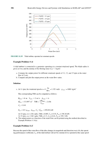
FIGURE 11.19 Tidal turbine operated at constant speeds.

Example Problem 11.4

A tidal turbine is connected to a generator operating at a constant rotational speed. The blade radius is
given as 6 m, and the density of the flowing water is ρ = 1 kg/m .
3
a. Compute the output power for different rotational speeds of 11, 13, and 15 rpm at the water
flow of 2 m/s.
b. Compute and plot the output power as the water flow varies.

Solution

2 π
a. At 11 rpm, the rotational speed ω:=11 = . 1 152 rad/s ρ water :=1000 kg/m 3
60 s
The corresponding TSR can be computed as follows:

π
R blade := 6 m V water := 2 m s A swept :=⋅
/
ω
2
R blade =113 .097 m 2 TSR := R blaade = 3 456
.
V water
C p = 044: .
P out := 05 ρ water ⋅ A swept ⋅ CV water =199 .051 kW
. ⋅
p ⋅
3
At 13 rpm, ω = 1.361 rad/s, TSR = 4.085, C p = 0.35, P out = 158.34 kW.
At 15 rpm, ω = 1.361 rad/s, TSR = 4.71, C p = 0.44, P out = 199.1 kW.
b. The output power as a function of the water flow can be plotted using the method described in
Example Problem 11.4(a).
Example Problem 11.5

Because the speed of the water flow of the tides changes in magnitude and direction every 6 h, the operat-
ing performance coefficient, C p , of the tidal turbine will not be constant if it is operated at the same speed