Page 172 - Reservoir Geomechanics

155 Faults and fractures at depth

a. b.
Active shear planes S 1
t Mode 2 and Mode 3
P
m = 0.6
m = 1.0 b
P 1 FAULT
b 3
S
2b 2
3 2b 1
S
s 3 s 2 s 1 n S 3
Mode 1
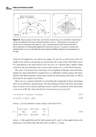
Figure 5.9. Representation of the shear and effective normal stress on an arbitrarily oriented fault
can be accomplished with a three-dimensional Mohr circle (a). Although the exact position of
point P can be determined with angles β 1 and β 3 measured between the fault normal and S 1
and S 3 directions (b) utilizing the graphical reconstruction shown, it is typical to calculate this
mathematically (see text) and utilize the three-dimensional Mohr diagram for representation of
the data.

location of P graphically, one utilizes the angles 2β 1 and 2β 3 to find points on the two
small circles, and by constructing arcs drawn from the center of the other Mohr circle,
Pis determined as the intersection of the two arcs. It is obvious that a Mode I plane
(normal to the least principal stress) plots at the position of σ 3 in the Mohr diagram.
Of course, it is not necessary these days to use graphical techniques alone for deter-
mining the shear and effective normal stress on arbitrarily oriented planes, but three-
dimensional Mohr diagrams remain quite useful for representing fault data, as will be
illustrated in the chapters that follow.
There are two common methods for calculating the magnitude of shear and normal
stress on an arbitrarily oriented plane. The first technique defines the shear and normal
stress in terms of the effective principal stresses and the orientation of the fault plane
to the stress field. The shear and effective normal stresses are given by

(5.7)
τ = a 11 a 12 σ 1 + a 12 a 22 σ 2 + a 13 a 23 σ 3
2 2 2
σ n = a σ 1 + a σ 2 + a σ 3 (5.8)
11 12 13
where a ij are the direction cosines (Jaeger and Cook 1971):

 
cos γ cos λ cos γ sin λ −sin γ
−sin λ cos λ 0 (5.9)
 
A = 

sin γ cos λ sin γ sin λ cos γ
where γ is the angle between the fault normal and S 3 , and λ is the angle between the
projection of the fault strike direction and S 1 in the S 1 –S 2 plane.