Page 169 - Reservoir Geomechanics

152 Reservoir geomechanics

a.
Tadpole plot b. N
0 30 60 90
6500 POLES TO
FRACTURE LANES

W E

6600

S
c. N
KAMB CONTOUR
OF POLES TO PLANES
6700
MAX. DENSIT Y = 4.76 sd
Depth (ft MD) W E

6800
0 0.4 0.8 1.2 1.6 2 2.4 2.8 3.2 3.6 4 4.4
S
d. N

FRACTURE STRIKE
6900
N = 1,987
W E

7000
S
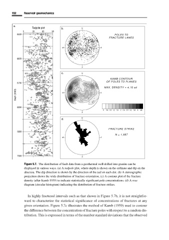
Figure 5.7. The distribution of fault data from a geothermal well drilled into granite can be
displayed in various ways. (a) A tadpole plot, where depth is shown on the ordinate and dip on the
abscissa. The dip direction is shown by the direction of the tail on each dot. (b) A stereographic
projection shows the wide distribution of fracture orientation. (c) A contour plot of the fracture
density (after Kamb 1959)to indicate statistically significant pole concentrations. (d) A rose
diagram (circular histogram) indicating the distribution of fracture strikes.

In highly fractured intervals such as that shown in Figure 5.7b, it is not straightfor-
ward to characterize the statistical significance of concentrations of fractures at any
given orientation. Figure 5.7c illustrates the method of Kamb (1959) used to contour
the difference between the concentration of fracture poles with respect to a random dis-
tribution. This is expressed in terms of the number standard deviations that the observed