Page 168 - Reservoir Geomechanics

151 Faults and fractures at depth

a. b. Shallow NW and SW
STRIKE
o
N N30 E dipping planes
N
W E 2
3
S
DIP W + 1 E
40 o 2
3
N N
30 o 1

Pole S
W + E
W E
40 o

S
S Cluster of SW dipping planes

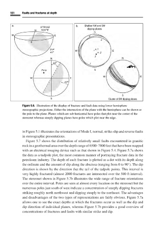
Figure 5.6. Illustration of the display of fracture and fault data using lower hemisphere
stereographic projections. Either the intersection of the plane with the hemisphere can be shown or
the pole to the plane. Planes which are sub-horizontal have poles that plot near the center of the
stereonet whereas steeply dipping planes have poles which plot near the edge.

in Figure 5.1 illustrates the orientations of Mode I, normal, strike-slip and reverse faults
in stereographic presentations.
Figure 5.7 shows the distribution of relatively small faults encountered in granitic
rock in a geothermal area over the depth range of 6500–7000 feet that have been mapped
with an electrical imaging device such as that shown in Figure 5.4. Figure 5.7a shows
the data as a tadpole plot, the most common manner of portraying fracture data in the
petroleum industry. The depth of each fracture is plotted as a dot with its depth along
the ordinate and the amount of dip along the abscissa (ranging from 0 to 90 ). The dip
◦
direction is shown by the direction that the tail of the tadpole points. This interval is
very highly fractured (almost 2000 fractures are intersected over the 500 ft interval).
The stereonet shown in Figure 5.7b illustrates the wide range of fracture orientations
over the entire interval. Poles are seen at almost every location on the stereonet but the
numerous poles just south of west indicate a concentration of steeply dipping fractures
striking roughly north northwest and dipping steeply to the northeast. The advantages
and disadvantages of the two types of representations are fairly obvious. Figure 5.7a
allows one to see the exact depths at which the fractures occur as well as the dip and
dip direction of individual planes, whereas Figure 5.7b provides a good overview of
concentrations of fractures and faults with similar strike and dip.