Page 190 -

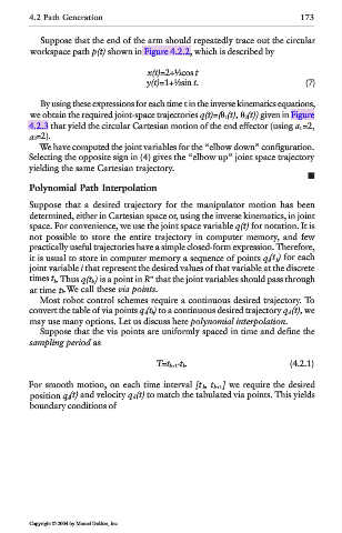
4.2 Path Generation 173

Suppose that the end of the arm should repeatedly trace out the circular
workspace path p(t) shown in Figure 4.2.2, which is described by

x(t)=2+½cos t
y(t)=1+½sin t. (7)

By using these expressions for each time t in the inverse kinematics equations,
we obtain the required joint-space trajectories q(t)=( 1 (t), 2 (t)) given in Figure
4.2.3 that yield the circular Cartesian motion of the end effector (using a 1 =2,
a 2 =2).
We have computed the joint variables for the “elbow down” configuration.
Selecting the opposite sign in (4) gives the “elbow up” joint space trajectory
yielding the same Cartesian trajectory.

Polynomial Path Interpolation
Suppose that a desired trajectory for the manipulator motion has been
determined, either in Cartesian space or, using the inverse kinematics, in joint
space. For convenience, we use the joint space variable q(t) for notation. It is
not possible to store the entire trajectory in computer memory, and few
practically useful trajectories have a simple closed-form expression. Therefore,
it is usual to store in computer memory a sequence of points q i (t k ) for each
joint variable i that represent the desired values of that variable at the discrete
n
times t k. Thus q(t k) is a point in R that the joint variables should pass through
at time t k.We call these via points.
Most robot control schemes require a continuous desired trajectory. To
convert the table of via points q i(t k) to a continuous desired trajectory q d(t), we
may use many options. Let us discuss here polynomial interpolation.
Suppose that the via points are uniformly spaced in time and define the
sampling period as

T=t k+1-t k. (4.2.1)

For smooth motion, on each time interval [t k, t k+1] we require the desired
.
position q d(t) and velocity q d(t) to match the tabulated via points. This yields
boundary conditions of

Copyright © 2004 by Marcel Dekker, Inc.