Page 193 -

176 Computed-Torque Control

Although we have used the joint variable notation q(t), it should be
emphasized that trajectory interpolation can also be performed in Cartesian
space.
Linear Function with Parabolic Blends

Using cubic interpolating polynomials, the acceleration on each sample
period is linear. However, in many practical applications there are good
reasons for insisting on constant accelerations within each sample period.
For instance, any real robot has upper limits on the torques that can be
supplied by its actuators. For linear systems (think of Newton’s law) this
translates into constant accelerations. Therefore, constant accelerations are
less likely to saturate the actuators. Besides that, most industrial robot
controllers are programmed to use constant accelerations on each sample
period.
A constant acceleration profile is shown in Figure 4.2.4(a). The associated
velocity and position profiles are shown in Figure 4.2.4(b) and 4.2.4(c). The
position trajectory has three parts: a quadratic or parabolic initial portion,
a linear midsection, and a parabolic final portion. Therefore, let us discuss
interpolation of via points using linear functions with parabolic blends (LFPB).
The time at which the position trajectory switches from parabolic to
linear is known as the blend time t b . A position q di (t) should be specified for
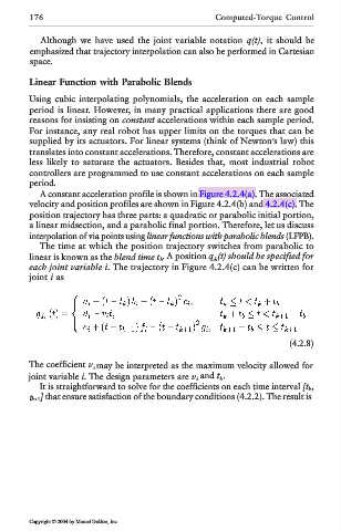
each joint variable i. The trajectory in Figure 4.2.4(c) can be written for
joint i as

(4.2.8)

The coefficient v i may be interpreted as the maximum velocity allowed for
joint variable i. The design parameters are v i and t b.
It is straightforward to solve for the coefficients on each time interval [t k,
t k+1] that ensure satisfaction of the boundary conditions (4.2.2). The result is

Copyright © 2004 by Marcel Dekker, Inc.