Page 192 -

4.2 Path Generation 175

(4.2.2)

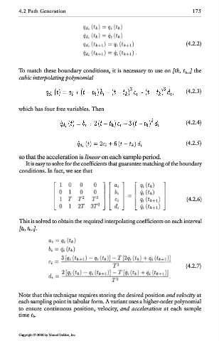
To match these boundary conditions, it is necessary to use on [tk, t k+1] the
cubic interpolating polynomial

(4.2.3)

which has four free variables. Then

(4.2.4)

(4.2.5)

so that the acceleration is linear on each sample period.
It is easy to solve for the coefficients that guarantee matching of the boundary
conditions. In fact, we see that

(4.2.6)

This is solved to obtain the required interpolating coefficients on each interval
[t k, t k+1].

(4.2.7)

Note that this technique requires storing the desired position and velocity at
each sampling point in tabular form. A variant uses a higher-order polynomial
to ensure continuous position, velocity, and acceleration at each sample
time t k.

Copyright © 2004 by Marcel Dekker, Inc.