Page 406 - Schaum's Outline of Theory and Problems of Advanced Calculus

CHAP. 16] FUNCTIONS OF A COMPLEX VARIABLE 397

and the connecting point constitute a Riemann surface, and w 1 and w 2 are the branches of the function
each defined in one of the planes. (Since the space of complex variables is the complex plane, this
Riemann surface may be thought of as a flight of fancy that supports a rigorous analytic construction.)
To visualize this Riemann surface and perceive the single-valued character of the new function in it,
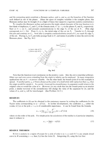
first think of duplicates, C 1 and C 2 of the domain circle, C: jzj¼ in the planes P 1 and P 2 , respectively.
Start at ¼ on C 1 , and proceed counterclockwise to the edge U 2 of the cut of P 1 . (This edge
corresponds to ¼ 2 ). Paste U 2 to L 1 , the initial edge of the cut on P 2 . Transfer to P 2 through
this join and continue on C 2 . Now after a complete counterclockwise circuit of C 2 we reach the edge L 2
of the cut. Pasting L 2 to U 1 provides passage back to P 1 and makes it possible to close the curve in the
Riemann plane. See Fig. 16-2.

Fig. 16-2

Note that the function is not continuous on the positive x-axis. Also the cut is somewhat arbitrary.
Other rays and even curves extending from the origin to infinity can be employed. In many integration
applications the cut ¼ i proves valuable. On the other hand, the branch point (0 in this example) is
special. If another point, z 0 6¼ 0 were chosen as the center of a small circle with radius less than jz 0 j, then
the origin would lie outside it. As a point z traversed its circumference, its argument would return to the
original value as would the value of w. However, for any circle that has the branch point as an interior
point, a similar traversal of the circumference will change the value of the argument by 2 , and the
values of w 1 and w 2 will be interchanged. (See Problem 16.37.)

RESIDUES
The coefficients in (9) can be obtained in the customary manner by writing the coefficients for the
n
Taylor series corresponding to ðz aÞ f ðzÞ. In further developments, the coefficient a 1 , called the
residue of f ðzÞ at the pole z ¼ a,isofconsiderable importance. It can be found from the formula
1 d n 1 n
a 1 ¼ lim
z!a ðn 1Þ! dz n 1 fðz aÞ f ðzÞg ð10Þ
where n is the order of the pole. For simple poles the calculation of the residue is of particular simplicity
since it reduces to

a 1 ¼ limðz aÞ f ðzÞ ð11Þ
z!a

RESIDUE THEOREM
If f ðzÞ is analytic in a region r except for a pole of order n at z ¼ a and if C is any simple closed
curve in r containing z ¼ a, then f ðzÞ has the form (9). Integrating (9), using the fact that