Page 49 - Schaum's Outline of Theory and Problems of Electric Circuits

ANALYSIS METHODS
38
4.2 THE MESH CURRENT METHOD [CHAP. 4

In the mesh current method a current is assigned to each window of the network such that the
currents complete a closed loop. They are sometimes referred to as loop currents. Each element and
branch therefore will have an independent current. When a branch has two of the mesh currents, the
actual current is given by their algebraic sum. The assigned mesh currents may have either clockwise or
counterclockwise directions, although at the outset it is wise to assign to all of the mesh currents a
clockwise direction. Once the currents are assigned, Kirchhoff’s voltage law is written for each loop to
obtain the necessary simultaneous equations.

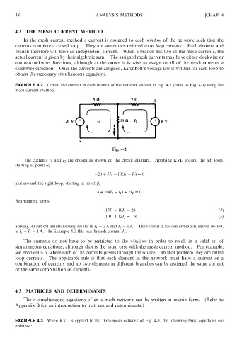
EXAMPLE 4.2 Obtain the current in each branch of the network shown in Fig. 4-2 (same as Fig. 4-1) using the
mesh current method.

Fig. 4-2

The currents I 1 and I 2 are chosen as shown on the circuit diagram. Applying KVL around the left loop,
starting at point ,
20 þ 5I 1 þ 10ðI 1 I 2 Þ¼ 0

and around the right loop, starting at point ,
8 þ 10ðI 2 I 1 Þþ 2I 2 ¼ 0
Rearranging terms,

15I 1 10I 2 ¼ 20 ð4Þ
10I 1 þ 12I 2 ¼ 8 ð5Þ

Solving (4) and (5) simultaneously results in I 1 ¼ 2 A and I 2 ¼ 1 A. The current in the center branch, shown dotted,
is I 1 I 2 ¼ 1 A. In Example 4.1 this was branch current I 3 .

The currents do not have to be restricted to the windows in order to result in a valid set of
simultaneous equations, although that is the usual case with the mesh current method. For example,
see Problem 4.6, where each of the currents passes through the source. In that problem they are called
loop currents. The applicable rule is that each element in the network must have a current or a
combination of currents and no two elements in different branches can be assigned the same current
or the same combination of currents.

4.3 MATRICES AND DETERMINANTS
The n simultaneous equations of an n-mesh network can be written in matrix form. (Refer to
Appendix B for an introduction to matrices and determinants.)

EXAMPLE 4.3 When KVL is applied to the three-mesh network of Fig. 4-3, the following three equations are
obtained: