Page 51 - Schaum's Outline of Theory and Problems of Electric Circuits

40
Similarly, ANALYSIS METHODS [CHAP. 4

1 R 11 V 1 R 13 1 R 11 R 12 V 1
I 2 ¼ R 21 V 2 R 23 I 3 ¼ R 21 R 22 V 2
R R
R 31 V 3 R 33 R 31 R 32 V 3
An expansion of the numerator determinants by cofactors of the voltage terms results in a set of equations
which can be helpful in understanding the network, particularly in terms of its driving-point and transfer resistances:

11 21 31
I 1 ¼ V 1 þ V 2 þ V 3 ð7Þ
R R R

12 22 32
I 2 ¼ V 1 þ V 2 þ V 3 ð8Þ
R R R

13 23 33
I 3 ¼ V 1 þ V 2 þ V 3 ð9Þ
R R R
Here, ij stands for the cofactor of R ij (the element in row i, column j)in R . Care must be taken with the
signs of the cofactors—see Appendix B.

4.4 THE NODE VOLTAGE METHOD
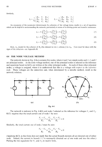
The network shown in Fig. 4-4(a) contains five nodes, where 4 and 5 are simple nodes and 1, 2, and 3
are principal nodes. In the node voltage method, one of the principal nodes is selected as the reference
and equations based on KCL are written at the other principal nodes. At each of these other principal
nodes, a voltage is assigned, where it is understood that this is a voltage with respect to the reference
node. These voltages are the unknowns and, when determined by a suitable method, result in the
network solution.

Fig. 4-4

The network is redrawn in Fig. 4-4(b) and node 3 selected as the reference for voltages V 1 and V 2 .
KCL requires that the total current out of node 1 be zero:

V 1 V a V 1 V 1 V 2
þ þ ¼ 0
R A R B R C
Similarly, the total current out of node 2 must be zero:

V 2 V 1 V 2 V 2 V b
þ þ ¼ 0
R C R D R E
(Applying KCL in this form does not imply that the actual branch currents all are directed out of either
node. Indeed, the current in branch 1–2 is necessarily directed out of one node and into the other.)
Putting the two equations for V 1 and V 2 in matrix form,