Page 50 - Schaum's Outline of Theory and Problems of Electric Circuits

CHAP. 4]

R B I 2
ðR A þ R B ÞI 1 ANALYSIS METHODS ¼ V a 39
R D I 3 ¼ 0
R B I 1 þðR B þ R C þ R D ÞI 2
R D I 2 þðR D þ R E ÞI 3 ¼ V b
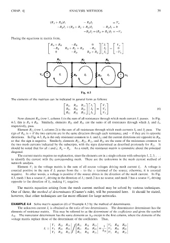
Placing the equations in matrix form,
2 32 3 2 3
R A þ R B R B 0 I 1 V a
4
4 R B R B þ R C þ R D R D 5 I 2 5 ¼ 4 0 5
0 R D R D þ R E I 3 V b

Fig. 4-3

The elements of the matrices can be indicated in general form as follows:
2 32 3 2 3
R 11 R 12 R 13 I 1 V 1
4
4 5 I 2 5 ¼ 4 5 ð6Þ
R 21 R 22 R 23 V 2
R 31 R 32 R 33 I 3 V 3
Now element R 11 (row 1, column 1) is the sum of all resistances through which mesh current I 1 passes. In Fig.
4-3, this is R A þ R B . Similarly, elements R 22 and R 33 are the sums of all resistances through which I 2 and I 3 ,
respectively, pass.
Element R 12 (row 1, column 2) is the sum of all resistances through which mesh currents I 1 and I 2 pass. The
sign of R 12 is þ if the two currents are in the same direction through each resistance, and if they are in opposite
directions. In Fig. 4-3, R B is the only resistance common to I 1 and I 2 ; and the current directions are opposite in R B ,
so that the sign is negative. Similarly, elements R 21 , R 23 , R 13 , and R 31 are the sums of the resistances common to
the two mesh currents indicated by the subscripts, with the signs determined as described previously for R 12 . It
should be noted that for all i and j, R ij ¼ R ji . As a result, the resistance matrix is symmetric about the principal
diagonal.
The current matrix requires no explanation, since the elements are in a single column with subscripts 1, 2, 3, . . .
to identify the current with the corresponding mesh. These are the unknowns in the mesh current method of
network analysis.
Element V 1 in the voltage matrix is the sum of all source voltages driving mesh current I 1 . A voltage is
counted positive in the sum if I 1 passes from the to the þ terminal of the source; otherwise, it is counted
negative. In other words, a voltage is positive if the source drives in the direction of the mesh current. In Fig.
4.3, mesh 1 has a source V a driving in the direction of I 1 ; mesh 2 has no source; and mesh 3 has a source V b driving
opposite to the direction of I 3 , making V 3 negative.
The matrix equation arising from the mesh current method may be solved by various techniques.
One of these, the method of determinants (Cramer’s rule), will be presented here. It should be stated,
however, that other techniques are far more efficient for large networks.

EXAMPLE 4.4 Solve matrix equation (6) of Example 4.3 by the method of determinants.
The unknown current I 1 is obtained as the ratio of two determinants. The denominator determinant has the
elements of resistance matrix. This may be referred to as the determinant of the coefficients and given the symbol
R . The numerator determinant has the same elements as R except in the first column, where the elements of the
voltage matrix replace those of the determinant of the coefficients. Thus,
,

V 1 R 12 R 13 R 11 R 12 R 13 1 V 1 R 12 R 13

I 1 ¼ V 2 R 22 R 23 R 21 R 22 R 23 V 2 R 22 R 23
R
V 3 R 32 R 33 R 31 R 32 R 33 V 3 R 32 R 33