Page 406 - Schaum's Outline of Theory and Problems of Signals and Systems

CHAP. 71 STATE SPACE ANALYSIS

First we expand H(s) in partial fractions as

1 3 I - 2 -
3
where H,(s) = - HZ(s) = - - H3(s) = - -
s+l s+2 s+5
yk(~)
ffk
Let Hk(s) = - -
=
s -Pk X(s)
Then (S -pk)Yk(s) =%X(S)
+
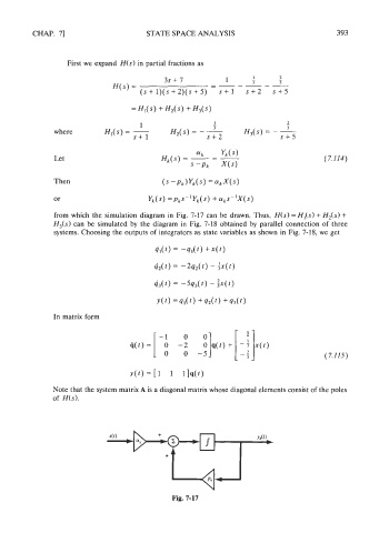
or Yk(s) =P~s-~Y~(s) aks-'X(s)
from which the simulation diagram in Fig. 7-17 can be drawn. Thus, H( S) = HJs) + H2(s) +
H,(s) can be simulated by the diagram in Fig. 7-18 obtained by parallel connection of three
systems. Choosing the outputs of integrators as state variables as shown in Fig. 7-18, we get

441) = -s,(t) +x(t)

&(t) = -2q~(t) - ;x(t)

q3(t) = -5q3(t) - :x(t)

~(t) =q,(t) +qz(t) +q,(t)

In matrix form

Note that the system matrix A is a diagonal matrix whose diagonal elements consist of the poles
of H(s).

Fig. 7-17