Page 405 - Schaum's Outline of Theory and Problems of Signals and Systems

392 STATE SPACE ANALYSIS [CHAP. 7

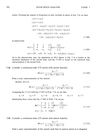
drawn. Choosing the outputs of integrators as state variables as shown in Fig. 7-16, we have
Cl(t) =u,(t)

In matrix form

As in the discrete-time case, the simulation of H(s) shown in Fig. 7-16 is known as the
canonical simulation of the second form, and Eq. (7.109) is known as the canonical state
representation of the second form.

7.18. Consider a continuous-time LTI system with system function

Find a state representation of the system.
Rewrite H(s) as

Comparing Eq. (7.111) with Eq. (7.105) in Prob. 7.16, we see that
a, =8 a, = 17 a, = 10 b,=b, =O b, = 3

Substituting these values into Eq. (7.106) in F 'rob. 7.16, we get

y(t) = [1 0 0

7.19. Consider a continuous-time LTI system with system function

Find a state representation of the system such that its system matrix A is diagonal.