
Page 403 - Schaum's Outline of Theory and Problems of Signals and Systems
P. 403
STATE SPACE ANALYSIS [CHAP. 7
From the definition of the system function [Eq. (3.37)]
we have
(s3 + als2 + a2s + a3)Y(s) = (bos3 + blsZ + b2s + b3)x(s)
Dividing both sides of the above expression by s3 and rearranging, we get
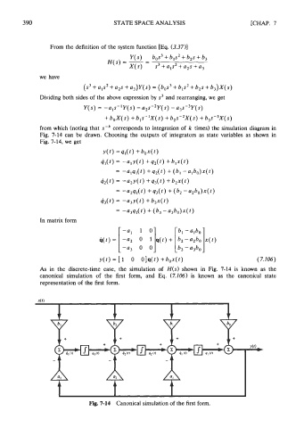
from which (noting that s-k corresponds to integration of k times) the simulation diagram in
Fig. 7-14 can be drawn. Choosing the outputs of integrators as state variables as shown in
Fig. 7-14, we get
As in the discrete-time case, the simulation of H(s) shown in Fig. 7-14 is known as the
canonical simulation of the first form, and Eq. (7.106) is known as the canonical state
representation of the first form.
Fig. 7-14 Canonical simulation of the first form.