Page 399 - Schaum's Outline of Theory and Problems of Signals and Systems

386 STATE SPACE ANALYSIS [CHAP. 7

In matrix form

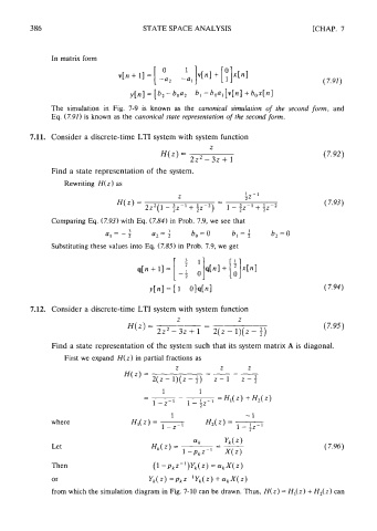
The simulation in Fig. 7-9 is known as the canonical simulation of the second form, and
Eq. (7.91) is known as the canonical state representation of the second form.

7.11. Consider a discrete-time LTI system with system function

H(z) =
2z2 - 3z + 1
Find a state representation of the system.
Rewriting H( z) as

Comparing Eq. (7.93) with Eq. (7.84) in Prob. 7.9, we see that

a =-2 =1
1 2 2 2 bo = 0 b, = f b2 = 0
Substituting these values into Eq. (7.85) in Prob. 7.9, we get

7.12. Consider a discrete-time LTI system with system function
Z - Z
H(z) = - (7.95)
2z2 - 32 + 1 2(z - l)(z - $)
Find a state representation of the system such that its system matrix A is diagonal.

First we expand H(z) in partial fractions as

where

Let

Then (1 -pkz-')Yk(z) =akX(z)

or Yk(z) =pkz-IYk(z) + akX(z)
from which the simulation diagram in Fig. 7-10 can be drawn. Thus, H( z) = HI( z) + H2( z ) can