Page 402 - Schaum's Outline of Theory and Problems of Signals and Systems

CHAP. 71 STATE SPACE ANALYSIS

7.15. Find state equations of a continuous-time LTI system described by
y(t) + 3y(t) + 2y(t) = 4x(t) +x(t) (7.103)
Because of the existence of the term 41(t) on the right-hand side of Eq. (7.103), the
selection of y(t) and y(t) as state variables will not yield the desired state equations of the
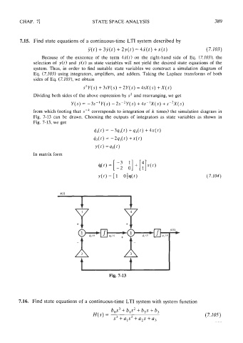
system. Thus, in order to find suitable state variables we construct a simulation diagram of
Eq. (7.103) using integrators, amplifiers, and adders. Taking the Laplace transforms of both
sides of Eq. (7.103), we obtain
+
s2~(s) 3sY(s) + 2Y(s) = 4sX(s) + X(s)
Dividing both sides of the above expression by s2 and rearranging, we get
+
+
Y(s) = -3Y1Y(s) - 2sC2~(s) 4s-'~(s) s-~x(s)
from which (noting that corresponds to integration of k times) the simulation diagram in
Fig. 7-13 can be drawn. Choosing the outputs of integrators as state variables as shown in

In matrix form

Fig. 7-13

7.16. Find state equations of a continuous-time LTI system with system function