Page 397 - Schaum's Outline of Theory and Problems of Signals and Systems

STATE SPACE ANALYSIS [CHAP. 7

From the definition of the system function [Eq. (4.4111

we have
(1 + a,z-' + ~,Z-~)Y(Z) = (6, + b,z-I + b,~-~)~(z)

Rearranging the above equation, we get
+
+
Y(z) = -a,z-'Y(z) -~,z-~Y(z) boX(z) + b,z-I~(z) b,~-~~(z)
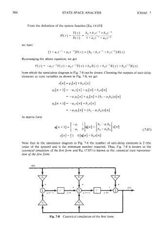
from which the simulation diagram in Fig. 7-8 can be drawn. Choosing the outputs of unit-delay
elements as state variables as shown in Fig. 7-8, we get

Y ~ I
=9,[nl +b,x[nl
q,[n + 11 = -a,y[nI + q2bI + b,x[nl

In matrix form

Note that in the simulation diagram in Fig. 7-8 the number of unit-delay elements is 2 (the
order of the system) and is the minimum number required. Thus, Fig. 7-8 is known as the
canonical simulation of the first form and Eq. (7.85) is known as the canonical state representa-
tion of the first form.

Fig. 7-8 canonical simulation of the first form.