Page 401 - Schaum's Outline of Theory and Problems of Signals and Systems
P. 401

388                            STATE SPACE ANALYSIS                            [CHAP.  7


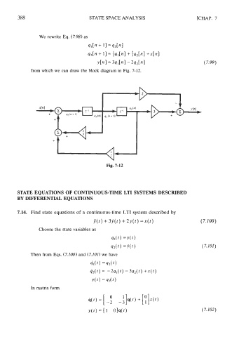
                    We rewrite  Eq.  (7.98) as
                                          4dn + 11 = qzbl

                                          q2[n + 11 = &l[n] + :q,[n] +x[n]
                                              Y ~ I3q,[nl - 2q2bI
                                                   =
                 from which we can draw the block diagram in  Fig. 7-12.


                                                  Fig. 7-12


           STATE EQUATIONS OF CONTINUOUS-TIME LTI SYSTEMS DESCRIBED
           BY DIFFERENTIAL EQUATIONS

           7.14.  Find state equations of a continuous-time LTI system described by

                                            y(t) + 3j(t) + 2y(t) =x(t)                      (7.100)
                    Choose the state variables as

                                                    sdt) =y(t)
                                                    92(1) =~(t)
                Then from Eqs. (7.100) and (7,101) we  have

                                           41(~) =q2(l)
                                           42(t)  = -2ql(f) -392(1) +x(t)
                                            Y(t) =4dt)
                 In matrix form
   396   397   398   399   400   401   402   403   404   405   406