Page 49 - Science at the nanoscale

RPS: PSP0007 - Science-at-Nanoscale
9:2
June 9, 2009
3.2. Basic Postulates of Quantum Mechanics
’
’
V=0
Ȍ
Ȍ
Ȍ
L
X
0
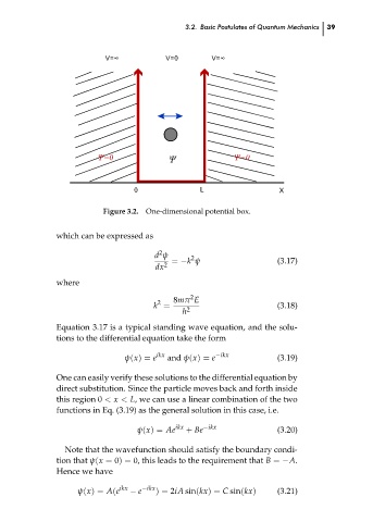
Figure 3.2. One-dimensional potential box.
which can be expressed as
2
d ψ
2
(3.17)
= −k ψ
2
dx
where
2
8mπ E
2
(3.18)
k =
2
h
Equation 3.17 is a typical standing wave equation, and the solu-
tions to the differential equation take the form
−ikx
ikx
ψ(x) = e
(3.19)
and ψ(x) = e
One can easily verify these solutions to the differential equation by 39 ch03
direct substitution. Since the particle moves back and forth inside
this region 0 < x < L, we can use a linear combination of the two
functions in Eq. (3.19) as the general solution in this case, i.e.
ψ(x) = Ae ikx + Be −ikx (3.20)
Note that the wavefunction should satisfy the boundary condi-
tion that ψ(x = 0) = 0, this leads to the requirement that B = −A.
Hence we have
ψ(x) = A(e ikx − e −ikx ) = 2iA sin(kx) = C sin(kx) (3.21)