Page 54 - Science at the nanoscale

9:2
RPS: PSP0007 - Science-at-Nanoscale
June 9, 2009
Brief Review of Quantum Mechanics
44
On the other hand, if L is large, the energy levels will be very
close to each other as depicted in Fig. 3.5(b). These closely spaced
energy levels practically form a continuous band and it is not
practical to account for each of these energy levels. It is more
practical to view the system by considering the number of energy
levels that can be found in a small energy range. This leads to the
idea of density of states and shall be discussed in Chapter 6.
Case 2: L x = L y = L and L z ≫ L x , L y . In such a case, the quan-
tisation condition (3.29) along the z-direction becomes essentially
continuous, i.e. there is only a small difference in k z and energy
for n z and n z + 1. Thus we can write the energy of the particle as
2
"
2
2
n
n
h
y
x
+ k
+
E =
2
2
L
L
8m
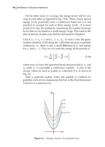
where now we have the quantised band characterised by n x and
n y while k z is essentially a continuous variable. A plot of the
energy values for such as system as a function of k z is shown in
Fig. 3.6.
Such a potential system where the particle is confined by
potential wells in two dimensions but free in the third dimension
is known as a quantum wire.
E
(1,3)
(2,2) 2 z # (3.32) ch03
(1,2)
(n ,n )=(1,1)
x y
k
z
Figure 3.6. Energy versus k z for quantum wire.