Page 125 - Semiconductor For Micro- and Nanotechnology An Introduction For Engineers

The Electronic System
variances as (3.9) and (3.10). We recall the transformation
⁄
q = — ( mω)ξ , thus we have the momentum operator given by
⁄
⁄
⁄
p ˆ = – i— ddq = ( mω) — ddξ . Since the potential is symmetric
about q = 0 we have q ˆ 〈〉 = 0 and p ˆ 〈〉 = 0 . We calculate q ˆ 〈 2 〉 and
p ˆ 〈 2 : 〉
∞
1
—
12∫
q ˆ 〈 2 〉 = ----------------------- exp  – ξ 2  2  – ξ 2  ξ 1 — (3.66a)
----- ξ exp
-----------
----- d =
mω π() ⁄  2   2  2mω
∞
∞
1  ξ 2  d 2  ξ 2  —mω
12∫
p ˆ 〈 2 〉 = – —mω--------------- exp – ----- --------exp – ----- d = ------------ (3.66b)
ξ
π () ⁄  2  dξ 2  2  2
∞
and thus their product yields
— 2
2
2
( 〈 ∆x ˆ) 〉 (〈 ∆p ˆ ) 〉 = p ˆ 〈 2 〉 q ˆ 〈 2 〉 = ----- (3.67)
4
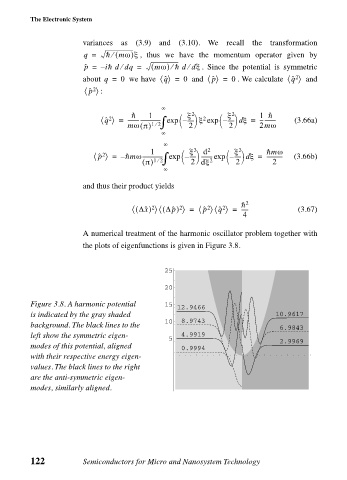
A numerical treatment of the harmonic oscillator problem together with
the plots of eigenfunctions is given in Figure 3.8.
25
20
Figure 3.8. A harmonic potential 15
12.9466
is indicated by the gray shaded 10.9617
10 8.9743
background. The black lines to the 6.9843
left show the symmetric eigen- 5 4.9919 2.9969
modes of this potential, aligned 0.9994
with their respective energy eigen-
values. The black lines to the right
are the anti-symmetric eigen-
modes, similarly aligned.

122 Semiconductors for Micro and Nanosystem Technology