Page 230 - Semiconductor For Micro- and Nanotechnology An Introduction For Engineers

From Global Balance to Local Non-Equilibrium
d
d
j
(
qD ---- Bu ([
[
(
kj
ki
ni
i
k
k
nj
i
L
L i jk )n – Bu )n ] + qD ----- Bu ( ik )n – Bu )n ]
i j
(6.98)
d L + d L j
i i
j
= qR --------------------------
k
2
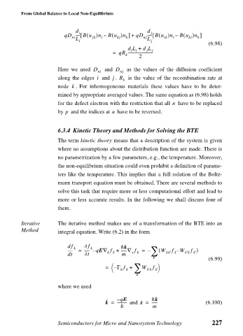
Here we used D and D as the values of the diffusion coefficient
ni nj
along the edges and . j R is the value of the recombination rate at
i
k
node . For inhomogeneous materials these values have to be deter-
k
mined by appropriate averaged values. The same equation as (6.98) holds
for the defect electron with the restriction that all have to be replaced
n
u
by and the indices at have to be reversed.
p
6.3.4 Kinetic Theory and Methods for Solving the BTE
The term kinetic theory means that a description of the system is given
where no assumptions about the distribution function are made. There is
no parametrization by a few parameters, e.g., the temperature. Moreover,
the non-equilibrium situation could even prohibit a definition of parame-
ters like the temperature. This implies that a full solution of the Boltz-
mann transport equation must be obtained. There are several methods to
solve this task that require more or less computational effort and lead to
more or less accurate results. In the following we shall discuss four of
them.
Iterative The iterative method makes use of a transformation of the BTE into an
Method integral equation. Write (6.2) in the form
df k ∂f k —k
f )
= – qE∇ f + ------∇ f = – ∑ ( W kk' k W k'k k'
f –
k k
x k
t d t ∂ m
k' (6.99)
 
k k ∑
= – Γ f + W f
 k'k k' 
k'
where we used
˙
----------
k = – qE and x ˙ = —k (6.100)
------
— m
Semiconductors for Micro and Nanosystem Technology 227