Page 232 - Semiconductor For Micro- and Nanotechnology An Introduction For Engineers

From Global Balance to Local Non-Equilibrium
Box 6.1. The Monte Carlo method.
Principle. The conduction of charge carriers
k
through a crystal is well approximated by a classi- x
cal free flight of the carrier under the influence of
x
its own momentum and the applied electromag-
netic fields, interspersed by scattering events
which change the momentum and energy of the
carrier. As we have seen, the scattering has many
causes, including the phonons, the impurity ions
and the other carriers.
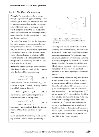
Figure B6.1.1. Typical 1D position and
The basis of the Monte Carlo method is to simu- momentum trajectories for the Monte Carlo
method.
late carrier transport by generating random scat-
tering events (hence the name Monte Carlo or series of pseudo random numbers: the onset of
MC) and numerically integrating the equations of scattering; the choice of scattering mechanism; the
motion of the carrier once the new momentum post-scattering momentum value; the post-scatter-
vector is known. Because in principle the MC ing momentum direction. The scattering events
needs to consider each carrier, and must collect typically included are: ionized impurity scattering,
enough data to be statistically relevant, it is very inter-valley absorption and emission and electron–
time consuming to calculate. phonon scattering. The terms also take into con-
Integration. During free flight over a time inter- sideration that the scattering rate is energy depen-
val the carriers behave classically, hence we can dent and that photons can be absorbed and
t
write the classical Newton relationship generated. In this way a high degree of realism is
achieved.
x t() = x 0() + tx ˙ 
 (B 6.1.1) Self-consistency. After initializing the simulation
p t() = p 0() + tF 
domain with carriers with position and momen-
for the position x t() and momentum p t() . The tum, the algorithm achieves a balance between
the force acting on a carrier is caused by the elec- classical electrostatics and the transport of carriers
tric field E acting on the carrier by the following repeated steps for each carrier:
τ
⁄
F t() = ∂p t() ∂t = q E (B 6.1.2) generate a lifetime ; compute the position x τ() -
c -
and momentum p τ() at the end of the free-flight
Just before the next collision, the position and
momentum have the following values step; select the next type of scattering event; com-
pute the post–scattering position x τ() + and
p t() = p 0() + q E +
c
(B 6.1.3) momentum p τ() ; decide if the trajectory has
⁄
x t() = x 0() + ∆E F
reached a boundary or contact, in which case it
for an energy increase of ∆E during the interval.
should be reflected or discontinued. If a contact is
Typical 1D trajectories are shown in Figure
reached, inject a new carrier at the complementary
B6.1.1.
contact; At regular intervals, recompute the elec-
Event generation. The scattering events are the tric field with the Poisson equation.
key to the MC method, and are generated by a
Semiconductors for Micro and Nanosystem Technology 229