Page 234 - Sensing, Intelligence, Motion : How Robots and Humans Move in an Unstructured World

PLANAR REVOLUTE–REVOLUTE (RR) ARM 209

simple circular obstacles, A, B, C, D (Figure 5.12). In spite of their simplicity,
we will see that moving between these obstacles turns out to be tricky.
As discussed before, at times both links of the arm may interact with obstacles
simultaneously, or one link may interact simultaneously with more than one
obstacle. For instance, when link l 1 touches obstacle D (Figure 5.12), obstacles
A and C maybeonthe wayoflink l 2 . Therefore, link l 2 may be touching at
least one of obstacles A or C, while at the same time link l 1 is touching obstacle
D. This means that in C-space, obstacles A, C,and D form a single obstacle.
Furthermore, note that if we position link l 2 between obstacles B and C and
start moving link l 1 past obstacle A, at some point link l 2 will simultaneously
touch obstacles B and C. In other words, in C-space all four obstacles create a
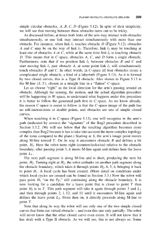
complicated single obstacle, a kind of a labyrinth (Figure 5.13). As it is formed
by two closed curves, this is a Type II obstacle. Also shown in Figure 5.13 is
the M-line (S, T ), chosen as a straight line in a “flatten” C-space.
Let us choose “right” as the local direction for the arm’s passing around an
obstacle. Although the sensing, the motion, and the actual algorithm procedure
will be happening in W-space, to understand what happens under this procedure
it is better to follow the generated path first in C-space. As we know already,
the reason C-space is easier to follow is that the C-space image of the path has
no self-intersections or double points, and obstacles are sets of simple closed
curves.
When watching it in C-space (Figure 5.13), one will recognize in the arm’s
path (indicated by arrows) the “signature” of the Bug2 procedure described in
Section 3.3.2. (We will see below that the resulting algorithm becomes more
complex than Bug2 because it has to take into account the more complex topology
of the torus compared to the plane.) Starting at S, the arm’s image point moves
along M-line toward T . On its way it encounters obstacle B and defines a hit
point, H 1 . Here the robot turns right (counterclockwise) relative to the obstacle
boundary; after passing point 3, it meets M-line again and defines here the leave
point L 1 .
The next path segment is along M-line and is short, producing the next hit
point, H 2 . Turning right at H 2 , the robot embarks on another path segment along
the obstacle boundary, which takes it through points H 2 , 6, 5, 4, bringing it back
to point H 1 . A local cycle has been created. (More detail on conditions under
which local cycles are created can be found in Section 3.3.) Now the robot will
pass point H 1 “on the fly,” still continuing along the obstacle boundary. It is
now looking for a candidate for a leave point that is closer to point T than
point H 2 is to T . This path segment will take it again through points 3 and L 1
and then through points 2, 1, 12, and 11 until it encounters M-line again and
defines the leave point L 2 . From then on, it directly proceeds along M-line to
point T .
Note that along its way the robot will see only one of the two simple closed
curves that form our virtual obstacle—and even this one only partially. The robot
will never know that the other closed curve even exists. It will not know that it
has dealt with a Type II obstacle. As we will see, this is not always so: Some