Page 252 - Sensing, Intelligence, Motion : How Robots and Humans Move in an Unstructured World

PRISMATIC–PRISMATIC (PP, OR CARTESIAN) ARM 227

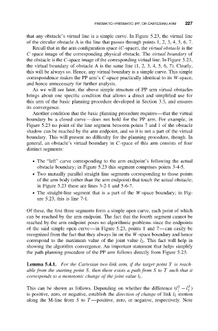
that any obstacle’s virtual line is a simple curve. In Figure 5.23, the virtual line
of the circular obstacle A is the line that passes through points 1, 2, 3, 4, 5, 6, 7.
Recall that in the arm configuration space (C-space), the virtual obstacle is the
C-space image of the corresponding physical obstacle. The virtual boundary of
the obstacle is the C-space image of the corresponding virtual line. In Figure 5.23,
the virtual boundary of obstacle A is the same line (1, 2, 3, 4, 5, 6, 7). Clearly,
this will be always so. Hence, any virtual boundary is a simple curve. This simple
correspondence makes the PP arm’s C-space practically identical to its W-space,
and hence unnecessary for further analysis.
As we will see later, the above simple structure of PP arm virtual obstacles
brings about one specific condition that allows a direct and simplified use for
this arm of the basic planning procedure developed in Section 3.3, and ensures
its convergence.
Another condition that the basic planning procedure requires—that the virtual
boundary be a closed curve—does not hold for the PP arm. For example, in
Figure 5.23 no point of the line segment between points 7 and 1 of the obstacle
shadow can be reached by the arm endpoint, and so it is not a part of the virtual
boundary. This will present no difficulty for the planning procedure, though. In
general, an obstacle’s virtual boundary in C-space of this arm consists of four
distinct segments:

• The “left” curve corresponding to the arm endpoint’s following the actual
obstacle boundary; in Figure 5.23 this segment comprises points 3-4-5.
• Two mutually parallel straight line segments corresponding to those points
of the arm body (other than the arm endpoint) that touch the actual obstacle;
in Figure 5.23 these are lines 3-2-1 and 5-6-7.
• The straight-line segment that is a part of the W-space boundary; in Fig-
ure 5.23, this is line 7-1.
Of these, the first three segments form a simple open curve, each point of which
can be reached by the arm endpoint. The fact that the fourth segment cannot be
reached by the arm endpoint poses no algorithmic problems since the endpoints
of the said simple open curve—in Figure 5.23, points 1 and 7—can easily be
recognized from the fact that they always lie on the W-space boundary and hence
correspond to the maximum value of the joint value l 2 . This fact will help in
showing the algorithm convergence. An important statement that helps simplify
the path planning procedure of the PP arm follows directly from Figure 5.23:

Lemma 5.4.1. For the Cartesian two-link arm, if the target point T is reach-
able from the starting point S, then there exists a path from S to T such that it
corresponds to a monotonic change of the joint value l 1 .

T
S
This can be shown as follows. Depending on whether the difference (l − l )
1 1
is positive, zero, or negative, establish the direction of change of link l 1 motion
along the M-line from S to T —positive, zero, or negative, respectively. Note