Page 55 - Sensing, Intelligence, Motion : How Robots and Humans Move in an Unstructured World

30 A QUICK SKETCH OF MAJOR ISSUES IN ROBOTICS

the arm somehow—say, acting upon the sensor data—arrives at some position,
from the arm’s joints we obtain its joint angles, and we would like to know
which position (x, y) in Cartesian space they correspond to (Figure 2.1). Hence
there is a need to translate from one coordinate system to the other.
Accordingly, there are two relationships between these two coordinate repre-
sentations:

Direct Kinematics. Given the values (θ 1 ,θ 1 ), find the corresponding Cartesian
coordinates (x, y) of the arm endpoint.
Inverse Kinematics. Given Cartesian coordinates (x, y) of the arm endpoint,
find the corresponding joint values (θ 1 ,θ 1 ).

∗
Note that if p is the vector from the proximal to the distal joint of link i
i
(Figure 2.2), i = 1, 2, then

cos θ 1
∗
p = l 1
1
sin θ 1
(2.1)

cos(θ 1 + θ 2 )
∗
p = l 2
2 sin(θ 1 + θ 2 )
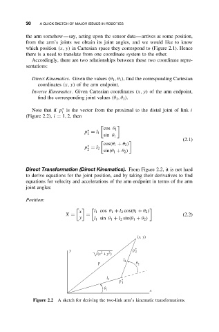
Direct Transformation (Direct Kinematics). From Figure 2.2, it is not hard
to derive equations for the joint position, and by taking their derivatives to find
equations for velocity and accelerations of the arm endpoint in terms of the arm
joint angles:

Position:

x l 1 cos θ 1 + l 2 cos(θ 1 + θ 2 )
X = = (2.2)
y l 1 sin θ 1 + l 2 sin(θ 1 + θ 2 )

(x, y)

y p ∗ 2
2
2
(x + y )
l 2
p q 2
l 1 ∗
p 1
q 1 x

Figure 2.2 A sketch for deriving the two-link arm’s kinematic transformations.