Page 64 - Sensing, Intelligence, Motion : How Robots and Humans Move in an Unstructured World

FEEDBACK CONTROL 39

q – q
d
K Disturbances
f, n
Commanded +
joint angle
e
q d − L + Σ Motor Robot Sensor
+ +
H
q
q

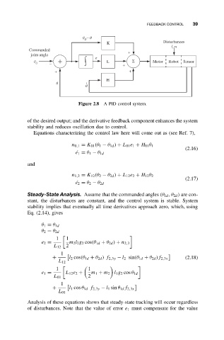
Figure 2.8 A PID control system.

of the desired output; and the derivative feedback component enhances the system
stability and reduces oscillation due to control.
Equations characterizing the control law here will come out as (see Ref. 7),

n 0,1 = K 01 (θ 1 − θ 1d ) + L 01 e 1 + H 01 θ 1
(2.16)
˙ e 1 = θ 1 − θ 1d

and

n 1,2 = K 12 (θ 2 − θ 2d ) + L 12 e 2 + H 12 θ 2
(2.17)
˙ e 2 = θ 2 − θ 2d
Steady-State Analysis. Assume that the commanded angles (θ 1d ,θ 2d ) are con-
stant, the disturbances are constant, and the control system is stable. System
stability implies that eventually all time derivatives approach zero, which, using
Eq. (2.14), gives

θ 1 = θ 1d
θ 2 = θ 2d
1 1
e 2 = m 2 l 2 g 2 cos(θ 1d + θ 2d ) + n 2,3
L 12 2
1
+ l 2 cos(θ 1d + θ 2d )f 2,3y − l 2 sin(θ 1d + θ 2d )f 2,3x (2.18)
L 12
1 1
e 1 = L 12 e 2 + m 1 + m 2 l 1 g 2 cos θ 1d
L 01 2
1
+ l 1 cos θ 1d f 2,3y − l 1 sin θ 1d f 2,3x
L 01
Analysis of these equations shows that steady-state tracking will occur regardless
of disturbances. Note that the value of error e 1 must compensate for the value