Page 61 - Sensing, Intelligence, Motion : How Robots and Humans Move in an Unstructured World

36 A QUICK SKETCH OF MAJOR ISSUES IN ROBOTICS

External Torques (Terms 5, 6, and 7). These are due to external forces and
torques that come from the arm’s interaction with other objects; they appear
when the arm physically touches objects, such as in assembly or cleaning.
During a free arm motion these torques are zeros.

Then there is another classification of dynamic torques, also with three types:
Inertial Torques. These are proportional to accelerations in the arm joints, and
they arise from normal action/reaction forces of an accelerating body.
Centripetal Torques. These torques arise from a constrained rotation about a
point, and they are proportional to the squares of joints’ velocities. For
example, the arm’s forearm must rotate about the arm’s shoulder joint, and
so the centripetal acceleration is aimed at the shoulder joint along link l 1
(Figure 2.1).
Coriolis Torques. These torques arise from vortical forces, as a result of inter-
action between two rotating systems (in our case two arm links), and they
are proportional to the product of joint velocities of two different links.
Notice the remarkable growth in the complexity of equations as we proceed
from kinematics to statics to dynamics equations. Then there is another natural
source of complexity—the arm complexity, measured by the number of robot
degrees of freedom. The reader is reminded that in our example, Figure 2.1, we
are dealing with the simplest two-link planar manipulator: In its analysis we
started with modest kinematic equations (2.2) and (2.3) and arrived at rather
complex dynamic equations in (2.14). Will the equations complexity grow as
quickly with the growth in the number of robot DOF?
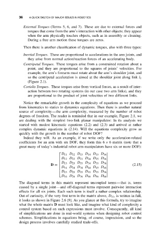
Indeed they will. As an example, if we write only the acceleration-related
coefficients for an arm with six DOF, they form this 6 × 6 matrix (note that a
great many of today’s industrial robot arm manipulators have six or more DOF):


D 11 D 12 D 13 D 14 D 15 D 16

D 12 D 22 D 23 D 24 D 25 D 26

(2.15)
D 13 D 23 D 33 D 34 D 35 D 36
D = 
D 14 D 24 D 34 D 44 D 45 D 46
 D 15 D 25 D 35 D 45 D 55 D 56

D 16 D 26 D 36 D 46 D 56 D 66
The diagonal terms in this matrix represent uncoupled terms—that is, terms
caused by a single joint—and off-diagonal terms represent pairwise interaction
effects for all six joints. Each such term is itself a rather complex relationship.
Out of curiosity, if the very first term in the matrix above, D 11 , is written in full,
it looks as shown in Figure 2.6 [9]. As you glance at this formula, try to imagine
what thewholematrix D must look like, and imagine what kind of complexity a
control system based on such expressions must involve. Consequently, all kind
of simplifications are done in real-world systems when designing robot control
schemes. Simplifications in equations bring, of course, imprecision, and so the
design process involves carefully studied trade-offs.