Page 314 - Separation process engineering

and Malone, 2001) is an example of the residue curves that occur in azeotropic distillation with added
solvent. The systems shown in Figures 8-11c and 8-12 are often formed on purpose by adding a solvent to
a binary azeotropic system.

Figure 8-11. Schematics of residue curve maps when there is one binary minimum-boiling azeotrope
(Doherty and Malone, 2001); reprinted with permission of McGraw-Hill, copyright 2001, McGraw-
Hill.

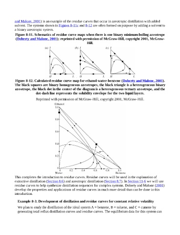
Figure 8-12. Calculated residue curve map for ethanol-water-benzene (Doherty and Malone, 2001).
The black squares are binary homogeneous azeotropes, the black triangle is a heterogeneous binary
azeotrope, the black dot in the center of the diagram is a heterogeneous ternary azeotrope, and the
dot-dash line represents the solubility envelope for the two liquid layers.

Reprinted with permission of McGraw-Hill, copyright 2001, McGraw-Hill.

This completes the introduction to residue curves. Residue curves will be used in the explanation of
extractive distillation (Section 8.6) and azeotropic distillation (Section 8.7). In Section 11-6 we will use
residue curves to help synthesize distillation sequences for complex systems. Doherty and Malone (2001)
develop the properties and applications of residue curves in much more detail than can be done in this
introduction.

Example 8-3. Development of distillation and residue curves for constant relative volatility
We plan to study the distillation of the ideal system A = benzene, B = toluene, and C = cumene by

generating total reflux distillation curves and residue curves. The equilibrium data for this system can