Page 65 - Separation process engineering

(2-4)

where F = degrees of freedom, C = number of components, and P = number of phases. For the binary
system in Table 2-1, C = 2 (ethanol and water) and P = 2 (vapor and liquid). Thus,

F = 2 − 2 + 2 = 2
When pressure and temperature are set, all the degrees of freedom are used, and at equilibrium all
compositions are determined from the experiment. Alternatively, we could set pressure and x Etoh or x w

and determine temperature and the other mole fractions.
The amount of material and its flow rate are not controlled by the Gibbs’ phase rule. The phase rule refers
to intensive variables such as pressure, temperature, or mole fraction, which do not depend on the total
amount of material present. The extensive variables, such as number of moles, flow rate, and volume, do

depend on the amount of material and are not included in the degrees of freedom. Thus a mixture in
equilibrium must follow Table 2-1 whether there are 0.1, 1.0, 10, 100, or 1,000 moles present.
Binary systems with only two degrees of freedom can be conveniently represented in tabular or graphical
form by setting one variable (usually pressure) constant. VLE data have been determined for many binary
systems. Sources for these data are listed in Table 2-2; you should become familiar with several of these
sources. Note that the data are not of equal quality. Methods for testing the thermodynamic consistency of
equilibrium data are discussed in detail by Barnicki (2002), Walas (1985), and Van Ness and Abbott
(1982, pp. 56–64, 301–348). Errors in the equilibrium data can have a profound effect on the design of

the separation method (e.g., see Carlson, 1996, or Nelson et al., 1983).

2.3 Graphical Representation of Binary VLE

Binary VLE data can be represented graphically in several ways. The most convenient forms are
temperature-composition, y-x, and enthalpy-composition diagrams. These figures all represent the same
data and can be converted from one form to another.

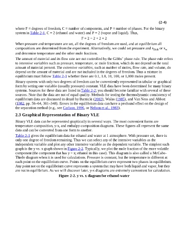
Table 2-1 gives the equilibrium data for ethanol and water at 1 atmosphere. With pressure set, there is
only one degree of freedom remaining. Thus we can select any of the intensive variables as the
independent variable and plot any other intensive variable as the dependent variable. The simplest such
graph is the y vs. x graph shown in Figure 2-2. Typically, we plot the mole fraction of the more volatile
component (the component that has y > x; ethanol in this case). This diagram is also called a McCabe-
Thiele diagram when it is used for calculations. Pressure is constant, but the temperature is different at
each point on the equilibrium curve. Points on the equilibrium curve represent two phases in equilibrium.
Any point not on the equilibrium curve represents a system that may have both liquid and vapor, but they
are not in equilibrium. As we will discover later, y-x diagrams are extremely convenient for calculation.

Figure 2-2. y vs. x diagram for ethanol-water