Page 310 - Shigley's Mechanical Engineering Design

bud29281_ch06_265-357.qxd 11/30/2009 4:23 pm Page 285 pinnacle s-171:Desktop Folder:Temp Work:Don't Delete (Jobs):MHDQ196/Budynas:

Fatigue Failure Resulting from Variable Loading 285
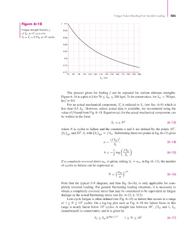
Figure 6–18 f 0.9

Fatigue strength fraction, f, 0.88
3
of S ut at 10 cycles for
6
S e = S = 0.5S ut at 10 cycles. 0.86

e
0.84
0.82

0.8
0.78

0.76
70 80 90 100 110 120 130 140 150 160 170 180 190 200
, kpsi
S ut

The process given for finding f can be repeated for various ultimate strengths.
Figure 6–18 is a plot of f for 70 ≤ S ut ≤ 200 kpsi. To be conservative, for S ut < 70 kpsi,
let f = 0.9.

For an actual mechanical component, S is reduced to S e (see Sec. 6–9) which is
e
less than 0.5 S ut . However, unless actual data is available, we recommend using the
value of f found from Fig. 6–18. Equation (a), for the actual mechanical component, can
be written in the form
S f = aN b (6–13)
3
where N is cycles to failure and the constants a and b are defined by the points 10 ,
6

S f 3 and 10 , S e with S f 3 = fS ut . Substituting these two points in Eq. (6–13) gives
10 10
( fS ut ) 2
a = (6–14)
S e
1 fS ut
b =− log (6–15)
3 S e
If a completely reversed stress σ rev is given, setting S f = σ rev in Eq. (6–13), the number
of cycles-to-failure can be expressed as

1/b
σ rev

N = (6–16)
a
Note that the typical S-N diagram, and thus Eq. (6–16), is only applicable for com-
pletely reversed loading. For general fluctuating loading situations, it is necessary to
obtain a completely reversed stress that may be considered to be equivalent in fatigue
damage as the actual fluctuating stress (see Ex. 6–12, p. 313).
Low-cycle fatigue is often defined (see Fig. 6–10) as failure that occurs in a range
3
of 1 ≤ N ≤ 10 cycles. On a log-log plot such as Fig. 6–10 the failure locus in this
3 3
range is nearly linear below 10 cycles. A straight line between 10 , fS ut and 1, S ut
(transformed) is conservative, and it is given by
S f ≥ S ut N (log f )/3 1 ≤ N ≤ 10 3 (6–17)