Page 218 -

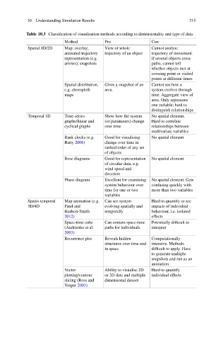
10 Understanding Simulation Results 215

Table 10.3 Classification of visualisation methods according to dimensionality and type of data
Method Pro Con
Spatial 1D/2D Map: overlay; View of whole Cannot analyse
animated trajectory trajectory of an object trajectory of movement.
representation (e.g. If several objects cross
arrows); snapshots paths, cannot tell
whether objects met at
crossing point or visited
points at different times
Spatial distribution, Gives a snapshot of an Cannot see how a
e.g. choropleth area. system evolves through
maps time. Aggregate view of
area. Only represents
one variable; hard to
distinguish relationships
Temporal 1D Time-series Show how the system No spatial element.
graphs/linear and (or parameters) change Hard to correlate
cyclical graphs over time relationships between
multivariate variables
Rank clocks (e.g. Good for visualising No spatial element
Batty 2006) change over time in
ranked order of any set
of objects
Rose diagrams Good for representation No spatial element
of circular data, e.g.
wind speed and
direction
Phase diagram Excellent for examining No spatial element. Gets
system behaviour over confusing quickly with
time for one or two more than two variables
variables
Spatio-temporal Map animation (e.g. Can see system Hard to quantify or see
3D/4D Patel and evolving spatially and impacts of individual
Hudson-Smith temporally behaviour, i.e. isolated
2012) effects
Space-time cube Can contain space-time Potentially difficult to
(Andrienko et al. paths for individuals interpret
2003)
Recurrence plot Reveals hidden Computationally
structures over time and intensive. Methods
in space difficult to apply. Have
to generate multiple
snapshots and run as an
animation
Vector Ability to visualise 2D Hard to quantify
plotting/contour or 3D data and multiple individual effects
slicing (Ross and dimensional dataset
Vosper 2003)