Page 306 -

13 Combining Mathematical and Simulation Approaches to Understand... 305

0.14
200 simulation runs
Empirical relative
0.12
frequency distribution
Relative frequency 0.08
0.10

0.06

0.04

0.02
0.00
75 80 85 90 95 100
Number of walkers in a house after 50 time-steps
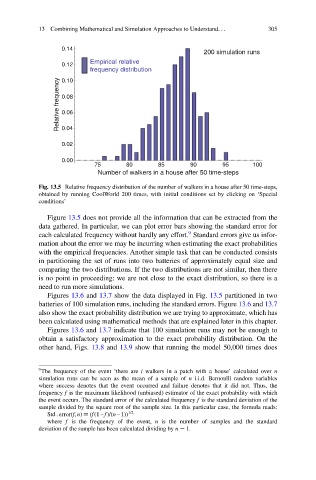
Fig. 13.5 Relative frequency distribution of the number of walkers in a house after 50 time-steps,
obtained by running CoolWorld 200 times, with initial conditions set by clicking on ‘Special
conditions’

Figure 13.5 does not provide all the information that can be extracted from the
data gathered. In particular, we can plot error bars showing the standard error for
9
each calculated frequency without hardly any effort. Standard errors give us infor-
mation about the error we may be incurring when estimating the exact probabilities
with the empirical frequencies. Another simple task that can be conducted consists
in partitioning the set of runs into two batteries of approximately equal size and
comparing the two distributions. If the two distributions are not similar, then there
is no point in proceeding: we are not close to the exact distribution, so there is a
need to run more simulations.
Figures 13.6 and 13.7 show the data displayed in Fig. 13.5 partitioned in two
batteries of 100 simulation runs, including the standard errors. Figure 13.6 and 13.7
also show the exact probability distribution we are trying to approximate, which has
been calculated using mathematical methods that are explained later in this chapter.
Figures 13.6 and 13.7 indicate that 100 simulation runs may not be enough to
obtain a satisfactory approximation to the exact probability distribution. On the
other hand, Figs. 13.8 and 13.9 show that running the model 50,000 times does

9 The frequency of the event ‘there are i walkers in a patch with a house’ calculated over n
simulation runs can be seen as the mean of a sample of n i.i.d. Bernoulli random variables
where success denotes that the event occurred and failure denotes that it did not. Thus, the
frequency f is the maximum likelihood (unbiased) estimator of the exact probability with which
the event occurs. The standard error of the calculated frequency f is the standard deviation of the
sample divided by the square root of the sample size. In this particular case, the formula reads:
Std . error(f, n) D (f(1 – f)/(n –1)) 1/2
where f is the frequency of the event, n is the number of samples and the standard
deviation of the sample has been calculated dividing by n 1.