Page 310 -

13 Combining Mathematical and Simulation Approaches to Understand... 309

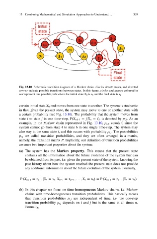
Fig. 13.10 Schematic transition diagram of a Markov chain. Circles denote states, and directed
arrows indicate possible transitions between states. In this figure, circles and arrows coloured in
red represent one possible path where the initial state X 0 is s 8 and the final state is s 2

certain initial state X 0 and moves from one state to another. The system is stochastic
in that, given the present state, the system may move to one or another state with
a certain probability (see Fig. 13.10). The probability that the system moves from
state i to state j in one time-step, P(X nC1 D jjX n D i), is denoted by p i,j .Asan
example, in the Markov chain represented in Fig. 13.10, p 4,6 equals 0 since the
system cannot go from state 4 to state 6 in one single time-step. The system may
also stay in the same state i, and this occurs with probability p i,i . The probabilities
p i,j are called transition probabilities, and they are often arranged in a matrix,
namely, the transition matrix P. Implicitly, our definition of transition probabilities
assumes two important properties about the system:
(a) The system has the Markov property. This means that the present state
contains all the information about the future evolution of the system that can
be obtained from its past, i.e. given the present state of the system, knowing the
past history about how the system reached the present state does not provide
any additional information about the future evolution of the system. Formally,

P .X nC1 D x nC1 jX n D x n ; X n–1 D x n–1 ;:::; X 0 D x 0 / D P .X nC1 D x nC1 jX n D x n /

(b) In this chapter we focus on time-homogeneous Markov chains, i.e. Markov
chains with time-homogeneous transition probabilities. This basically means
that transition probabilities p i,j are independent of time, i.e. the one-step
transition probability p i,j depends on i and j but is the same at all times n.
Formally,