Page 158 - Six Sigma Demystified

Chapter 6 a n a ly z e S tag e 139

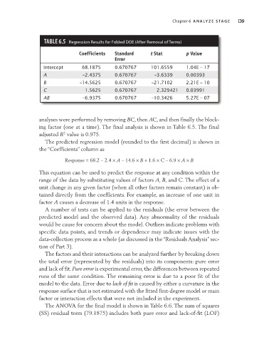
TAble­6.5­ Regression Results for Folded DOE (after Removal of Terms)

Coefficients Standard t Stat p Value
Error
Intercept 68.1875 0.670767 101.6559 1.04E – 17
A –2.4375 0.670767 –3.6339 0.00393
B –14.5625 0.670767 –21.7102 2.21E – 10
C 1.5625 0.670767 2.329421 0.03991
AB –6.9375 0.670767 –10.3426 5.27E – 07

analyses were performed by removing BC, then AC, and then finally the block-
ing factor (one at a time). The final analysis is shown in Table 6.5. The final
2
adjusted R value is 0.975.
The predicted regression model (rounded to the first decimal) is shown in
the “Coefficients” column as

Response = 68.2 – 2.4 × A – 14.6 × B + 1.6 × C – 6.9 × A × B

This equation can be used to predict the response at any condition within the
range of the data by substituting values of factors A, B, and C. The effect of a
unit change in any given factor (when all other factors remain constant) is ob-
tained directly from the coefficients. For example, an increase of one unit in
factor A causes a decrease of 1.4 units in the response.
A number of tests can be applied to the residuals (the error between the
predicted model and the observed data). Any abnormality of the residuals
would be cause for concern about the model. Outliers indicate problems with

specific data points, and trends or dependence may indicate issues with the
data- collection process as a whole (as discussed in the “Residuals Analysis” sec-
tion of Part 3).
The factors and their interactions can be analyzed further by breaking down
the total error (represented by the residuals) into its components: pure error
and lack of fit. Pure error is experimental error, the differences between repeated
runs of the same condition. The remaining error is due to a poor fit of the
model to the data. Error due to lack of fit is caused by either a curvature in the
response surface that is not estimated with the fitted first- degree model or main
factor or interaction effects that were not included in the experiment.
The ANOVA for the final model is shown in Table 6.6. The sum of squares
l
(SS) residual term (79.1875) includes both pure error and ack- of- fit (LOF)