Page 159 - Six Sigma Demystified

140 Six SigMa DemystifieD

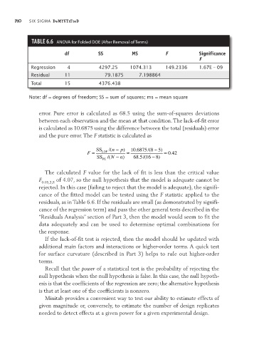
TAble­6.6­ aNOVa for Folded DOE (after Removal of Terms)

df SS MS F Significance
F
Regression 4 4297.25 1074.313 149.2336 1.67E – 09
Residual 11 79.1875 7.198864
Total 15 4376.438

Note: df = degrees of freedom; SS = sum of squares; ms = mean square

error. Pure error is calculated as 68.5 using the sum-of-squares deviations
between each observation and the mean at that condition. The lack- of- fit error
is calculated as 10.6875 using the difference between the total (residuals) error
and the pure error. The F statistic is calculated as

The calculated F value for the lack of fit is less than the critical value
F 0.05,3,8 of 4.07, so the null hypothesis that the model is adequate cannot be
rejected. In this case (failing to reject that the model is adequate), the signifi-
cance of the fitted model can be tested using the F statistic applied to the
residuals, as in Table 6.6. If the residuals are small (as demonstrated by signifi-
cance of the regression term) and pass the other general tests described in the
“Residuals Analysis” section of Part 3, then the model would seem to fit the
data adequately and can be used to determine optimal combinations for
the response.
If the ack- of- fit test is rejected, then the model should be updated with
l
additional main factors and interactions or higher- order terms. A quick test
for surface curvature (described in Part 3) helps to rule out higher- order
terms.
Recall that the power of a statistical test is the probability of rejecting the
null hypothesis when the null hypothesis is false. In this case, the null hypoth-
esis is that the coefficients of the regression are zero; the alternative hypothesis
is that at least one of the coefficients is nonzero.
Minitab provides a convenient way to test our ability to estimate effects of
given magnitude or, conversely, to estimate the number of design replicates
needed to detect effects at a given power for a given experimental design.