Page 404 - Six Sigma Demystified

384 Six SigMa DemystifieD

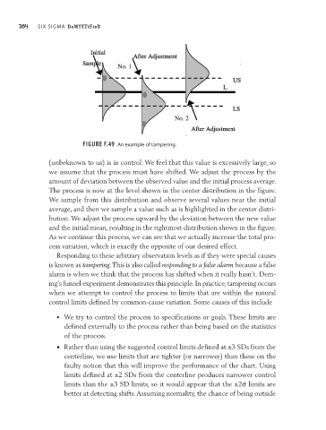
Figure F.49 an example of tampering.

(unbeknown to us) is in control. We feel that this value is excessively large, so
we assume that the process must have shifted. We adjust the process by the
amount of deviation between the observed value and the initial process average.
The process is now at the level shown in the center distribution in the figure.
We sample from this distribution and observe several values near the initial
average, and then we sample a value such as is highlighted in the center distri-
bution. We adjust the process upward by the deviation between the new value
and the initial mean, resulting in the rightmost distribution shown in the figure.
As we continue this process, we can see that we actually increase the total pro-
cess variation, which is exactly the opposite of our desired effect.
Responding to these arbitrary observation levels as if they were special causes
is known as tampering. This is also called responding to a false alarm because a false
alarm is when we think that the process has shifted when it really hasn’t. Dem-
ing’s funnel experiment demonstrates this principle. In practice, tampering occurs

when we attempt to control the process to limits that are within the natural
control limits defined by common-cause variation. Some causes of this include

• We try to control the process to specifications or goals. These limits are
defined externally to the process rather than being based on the statistics
of the process.
• Rather than using the suggested control limits defined at ±3 SDs from the
centerline, we use limits that are tighter (or narrower) than these on the
faulty notion that this will improve the performance of the chart. Using
limits defined at ±2 SDs from the centerline produces narrower control
limits than the ±3 SD limits, so it would appear that the ±2σ limits are
better at detecting shifts. Assuming normality, the chance of being outside