Page 120 - Six Sigma for electronics design and manufacturing

89
Six Sigma and Manufacturing Control Systems
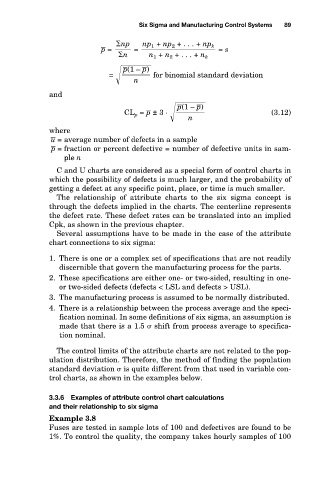
np
np 1 + np 2 + . . . + np k

n
n 1 + n 2 + . . . + n k

p(1 – p)

for binomial standard deviation
=

n
and

p(1 – p)

CL p = p ± 3 ·

n
where p = = = s (3.12)
u = average number of defects in a sample

p = fraction or percent defective = number of defective units in sam-

ple n
C and U charts are considered as a special form of control charts in
which the possibility of defects is much larger, and the probability of
getting a defect at any specific point, place, or time is much smaller.
The relationship of attribute charts to the six sigma concept is
through the defects implied in the charts. The centerline represents
the defect rate. These defect rates can be translated into an implied
Cpk, as shown in the previous chapter.
Several assumptions have to be made in the case of the attribute
chart connections to six sigma:
1. There is one or a complex set of specifications that are not readily
discernible that govern the manufacturing process for the parts.
2. These specifications are either one- or two-sided, resulting in one-
or two-sided defects (defects < LSL and defects > USL).
3. The manufacturing process is assumed to be normally distributed.
4. There is a relationship between the process average and the speci-
fication nominal. In some definitions of six sigma, an assumption is
made that there is a 1.5 shift from process average to specifica-
tion nominal.
The control limits of the attribute charts are not related to the pop-
ulation distribution. Therefore, the method of finding the population
standard deviation is quite different from that used in variable con-
trol charts, as shown in the examples below.
3.3.6 Examples of attribute control chart calculations
and their relationship to six sigma
Example 3.8
Fuses are tested in sample lots of 100 and defectives are found to be
1%. To control the quality, the company takes hourly samples of 100