Page 166 - Six Sigma for electronics design and manufacturing

135
The Use of Six Sigma with High- and Low-Volume Products and Processes
This distribution is always normal, even if the parent population dis-
tribution is not normal. It has also been shown the standard deviation
s of the distribution of sample averages is related to the parent distri-
bution standard deviation by the central limit theorem, which
states that s = / n (Equation 3.5). The number of samples needed to
construct the variable chart control limits was also set at a high level
of 20 successive samples to ensure that the population will be
known.
When the total number in the samples (n) is small, very little can be
determined by the sampling distribution for small values of n, unless
an assumption is made that the sample comes from a normal distribu-
tion. The normal distribution assumes an infinite number of occur-
rences that are represented by the process average and standard
deviation . The Student’s t distribution is used when n is small. The
data needed to construct this distribution are the sample average X
and sample standard deviation s, as well as the parent normal distri-
bution average :
X –
t = (5.1)
S/ n
where t is a random variable having the t distribution with = n – 1.
= degrees of freedom (DOF) = n – 1 (5.2)
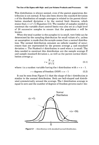
It can be seen from Figure 5.1 that the shape of the t distribution is
similar to the normal distribution. Both are bell-shaped and distrib-
uted symmetrically around the average. The t distribution average is
equal to zero and the number of degrees of freedom governs each t dis-

Figure 5.1 t distribution with standard normal distribution.