Page 170 - Six Sigma for electronics design and manufacturing

The Use of Six Sigma with High- and Low-Volume Products and Processes
139
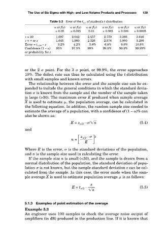
Table 5.2 Error of the t , of student’s t distribution
or f(z)
or f(z)
or f(z)
or f(z)
or f(z)
or f(z)
0.01
= 0.0005
= 0.005
= 0.001
= 0.025
= 0.05
2.042
1.697
2.457
2.750
3.646
3.386
= 30
1.645
3.290
= or z
2.326
2.576
1.960
3.090
3.2%
9.6%
4.2%
10.8%
5.6%
6.8%
Error = t ,30 – z
97.5%
99.95%
99.9%
Confidence (1 – )
99%
99.5%
95%
or probability for z
or the 2 point. For the 3 point, or 99.9%, the error approaches
10%. The defect rate can thus be calculated using the t-distribution
with small samples and known errors.
The relationship between the error and the sample size can be ex-
panded to include the general conditions in which the standard devia-
tion is known from the sample and the number of the sample taken
is large (>30). The maximum error E produced when sample average
X is used to estimate , the population average, can be calculated in
the following equation. In addition, the random sample size needed to
estimate the average of a population, with a confidence of (1 – )% can
also be shown as:
E = z /2 · / n (5.4)
and
z /2 ·
2
n =
E
Where E is the error, is the standard deviations of the population,
and n is the sample size used in calculating the error.
If the sample size n is small (<30), and the sample is drawn from a
normal distribution of the population, the standard deviation of popu-
lation is not known, but the sample standard deviation s can be cal-
culated from the sample. In this case, the error made when the sam-
ple average X is used to estimate population average is as follows:
s
E = t /2 · (5.5)
n
5.1.3 Examples of point estimation of the average
Example 5.3
An engineer uses 100 samples to check the average noise output of
amplifiers (in dB) produced in the production line. If it is known that