Page 172 - Six Sigma for electronics design and manufacturing

141
The Use of Six Sigma with High- and Low-Volume Products and Processes

< X + z /2 ·
X – z /2 ·
<
(5.6)
n
n
and
s
s
X – t /2 ·
(5.7)
< X + t /2 ·
<
n
n
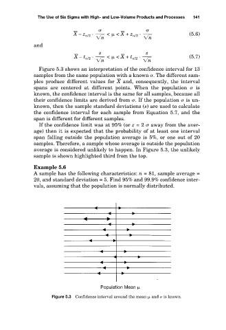
Figure 5.3 shows an interpretation of the confidence interval for 13
samples from the same population with a known . The different sam-
ples produce different values for X and, consequently, the interval
spans are centered at different points. When the population is
known, the confidence interval is the same for all samples, because all
their confidence limits are derived from . If the population is un-
known, then the sample standard deviations (s) are used to calculate
the confidence interval for each sample from Equation 5.7, and the
span is different for different samples.
If the confidence limit was at 95% (or z = 2 away from the aver-
age) then it is expected that the probability of at least one interval
span falling outside the population average is 5%, or one out of 20
samples. Therefore, a sample whose average is outside the population
average is considered unlikely to happen. In Figure 5.3, the unlikely
sample is shown highlighted third from the top.
Example 5.6
A sample has the following characteristics: n = 81, sample average =
20, and standard deviation = 5. Find 95% and 99.9% confidence inter-
vals, assuming that the population is normally distributed.

Population Mean
Figure 5.3 Confidence interval around the mean and is known.