Page 175 - Six Sigma for electronics design and manufacturing

Six Sigma for Electronics Design and Manufacturing
144
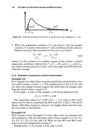
Figure 5.5 Obtaining confidence limits from distribution with confidence (1 – )%.
2
2
2. When the population variance is not known, and the sample
2
variance s is used to determine , with confidence limits and con-
2
fidence intervals. The equation for this case is as follows:
(n – 1)s 2 (n – 1)s 2
2
< < (5.9)
2 2
/2 1– /2
2
where s is the variance of a random sample of size n from a normal
2 2 2
population, confidence interval for is (1 – )%, and 1– /2 and – /2
are values having areas of /2 and – /2 to the right and left of the dis-
tribution average.
5.1.6 Examples of population variance determination
Example 5.8
Five samples are taken from a normal population of parts from a fac-
tory with average = 3 and = 1. The samples are 2.0, 2.5, 3.0, 3.5, and
4.0. Does this sample of parts support the belief that the sample came
from the factory with equal to 1?
X of sample = 3 and s of the sample = 0.79. From Equation (5.8)
2
2
= 4 · 0.79 /1 = 2.50
2
The calculated value of (2.50) with = 4 is close to 50% confi-
dence (3.357) and is in between the 90% and 10% (1.064–7.779) confi-
dences. Therefore, based on variance, it is highly likely that the sam-
ple was made at that factory.
Example 5.9
Nine samples (from Example 5.7) were taken from an assumed nor-
mal population with the following values from example: 5.7: 2.6, 2.1,
2.4, 2.5, 2.7, 2.2, 2.3, 2.4, and 1.9. What are the 95% and 99% confi-
dence intervals of population variance?
Sample data: n = 9; average = 2.34, and s = 0.25.