Page 83 - Six Sigma for electronics design and manufacturing

Six Sigma for Electronics Design and Manufacturing
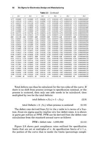
Table 2.3 Continued
f(z)
f(z)
z
z
z
z
f(z)
f(z)
z
z
f(z)
f(z)
–0.71
–2.72
0.23576 –1.72 0.04272
0.00326 –3.72
0.000100 –4.72 0.00000118 –5.72 0.00000000534
–0.72
–2.73
0.00317 –3.73
–0.73
0.23270 –1.73 0.04182
0.000096 –4.73 0.00000112 –5.73 0.00000000504
–0.74
0.000092 –4.74 0.00000107 –5.74 0.00000000475
0.22965 –1.74 0.04093
–2.74
0.00307 –3.74
–2.75
–0.75
0.00298 –3.75
0.000088 –4.75 0.00000102 –5.75 0.00000000448
0.22663 –1.75 0.04006
0.000085 –4.76 0.00000097 –5.76 0.00000000422
0.22363 –1.76 0.03920
–2.76
–0.76
0.00289 –3.76
0.22065 –1.77 0.03836
0.00280 –3.77
0.000082 –4.77 0.00000092 –5.77 0.00000000398
–2.77
–0.77
0.000078 –4.78 0.00000088 –5.78 0.00000000375
–2.78
0.00272 –3.78
0.21770 –1.78 0.03754
–0.78
–0.79
–2.79
0.000075 –4.79 0.00000083 –5.79 0.00000000353
0.21476 –1.79 0.03673
0.00264 –3.79
–2.8
0.00256 –3.8
0.000072 –4.8
0.00000000333
0.21186 –1.8
–0.8 52 0.23885 –1.71 0.04363 –2.71 0.00336 –3.71 0.000104 –4.71 0.00000124 –5.71 0.00000000567
0.00000079 –5.8
0.03593
–0.81 0.20897 –1.81 0.03515 –2.81 0.00248 –3.81 0.000070 –4.81 0.00000076 –5.81 0.00000000313
–0.82 0.20611 –1.82 0.03438 –2.82 0.00240 –3.82 0.000067 –4.82 0.00000072 –5.82 0.00000000295
–0.83 0.20327 –1.83 0.03362 –2.83 0.00233 –3.83 0.000064 –4.83 0.00000068 –5.83 0.00000000278
–0.84 0.20045 –1.84 0.03288 –2.84 0.00226 –3.84 0.000062 –4.84 0.00000065 –5.84 0.00000000262
–0.85 0.19766 –1.85 0.03216 –2.85 0.00219 –3.85 0.000059 –4.85 0.00000062 –5.85 0.00000000247
–0.86 0.19489 –1.86 0.03144 –2.86 0.00212 –3.86 0.000057 –4.86 0.00000059 –5.86 0.00000000232
–0.87 0.19215 –1.87 0.03074 –2.87 0.00205 –3.87 0.000054 –4.87 0.00000056 –5.87 0.00000000219
–0.88 0.18943 –1.88 0.03005 –2.88 0.00199 –3.88 0.000052 –4.88 0.00000053 –5.88 0.00000000206
–0.89 0.18673 –1.89 0.02938 –2.89 0.00193 –3.89 0.000050 –4.89 0.00000050 –5.89 0.00000000194
–0.9 0.18406 –1.9 0.02872 –2.9 0.00187 –3.9 0.000048 –4.9 0.00000048 –5.9 0.00000000182
–0.91 0.18141 –1.91 0.02807 –2.91 0.00181 –3.91 0.000046 –4.91 0.00000046 –5.91 0.00000000172
–0.92 0.17879 –1.92 0.02743 –2.92 0.00175 –3.92 0.000044 –4.92 0.00000043 –5.92 0.00000000162
–0.93 0.17619 –1.93 0.02680 –2.93 0.00169 –3.93 0.000042 –4.93 0.00000041 –5.93 0.00000000152
–0.94 0.17361 –1.94 0.02619 –2.94 0.00164 –3.94 0.000041 –4.94 0.00000039 –5.94 0.00000000143
–0.95 0.17106 –1.95 0.02559 –2.95 0.00159 –3.95 0.000039 –4.95 0.00000037 –5.95 0.00000000135
–0.96 0.16853 –1.96 0.02500 –2.96 0.00154 –3.96 0.000037 –4.96 0.00000035 –5.96 0.00000000127
–0.97 0.16602 –1.97 0.02442 –2.97 0.00149 –3.97 0.000036 –4.97 0.00000034 –5.97 0.00000000119
–0.98 0.16354 –1.98 0.02385 –2.98 0.00144 –3.98 0.000034 –4.98 0.00000032 –5.98 0.00000000112
–0.99 0.16109 –1.99 0.02330 –2.99 0.00139 –3.99 0.000033 –4.99 0.00000030 –5.99 0.00000000105
–1 0.15866 –2 0.02275 –3 0.00135 –4 0.000032 –5 0.00000029 –6 0.00000000099
Total defects can thus be calculated for the two sides of the curve. If
there is no shift from process average to specification nominal, or the
process is centered, then only one side needs to be calculated, then
multiplied by two for the total defects:
total defects = f(z 1 ) + 1 – f(z 2 ) (2.9)
total Defects = 2 · f(z 1 ) when process is centered (2.10)
The defect rate derived from f(z) in the z table is in terms of a frac-
tion. Since six sigma quality implies very low defect rates, it is shown
in parts per million or PPM. PPM can be derived from the defect rate
calculations from the standard normal curve as follows:
PPM = defect rate · 1,000,000 (2.11)
Figure 2.9 shows part compliance rates outlined for specification
limits that are set at multiples of . At specification limits of ± 1 ,
the portion of the curve that is inside the limits (percentage compli-