Page 79 - Six Sigma for electronics design and manufacturing

Six Sigma for Electronics Design and Manufacturing
48
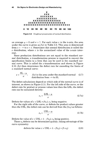
Figure 2.8 Graphical presentation of normal distribution.
an average = 0 and = 1. For each value z in the x-axis, the area
under the curve is given as f(z) in Table 2.3. This area is determined
from x = – to x = z. Sometimes this normal distribution is called the
z distribution, where z is the normalized value of the x-axis inter-
cept.
Since production distributions are not equal to the standard nor-
mal distribution, a transformation process is required to convert the
specification limits to a form that can be used in the standard nor-
mal curve. This is called the z-transformation and shown in Figure
2.10. f(z) then determines the defect rate for exceeding the limits of
a standard normal curve:
SL –
z = ; f(z) is the area under the standard normal (2.7)

distribution from – to SL
The defect calculations depend on which side of the normal curve is of
interest, as shown in Figure 2.11. For the left side of the curve, or the
defect rate for product or process values less then the LSL, the defect
rate can be calculated directly:

LSL –
z 1 = (2.7a)

Defects for values of z < LSL = f(z 1 ); z 1 being negative.
For the right side of the curve, or defects for product values greater
then the USL, the defect rate can be derived from the f(z 2 ) as follows:
USL –
z 2 = (2.7b)

Defects for value of z > USL = 1 – f(z 2 ); z 2 being positive.
These z 2 defects can be determined quickly, taking advantage of the
curve symmetry:
defects for value z > USL = 1 – f(z 2 ) = f(–z 2 ) (2.8)