Page 265 - Soil and water contamination, 2nd edition

252 Soil and Water Contamination

-1
-3
where k = zero-order rate constant [M L T ] which has a positive sign in the case of
0
production and a negative sign in the case of decay. Integration of this rate expression results
in a straight rising line for which the tangent of the slope equals the zero-order rate constant.
Note that if the production rate is expressed as a flux density , i.e. mass production per unit
area, the zero-order rate constant can be calculated as follows:
A
k J (13.23)
0
V
-2
2
-1
where J = flux density [M L T ], A = surface area over which production occurs [L ], and V =
3
volume of water body [L ]. The surface area divided by the water volume can be approximated
by 1/H where H = the water depth [L]. Then the differential equation becomes:
dC w J (13.24)
dt H
Combination of a zero-order production process (e.g. release of nutrients from bed
sediments ) and a first-order removal process yields the following differential equation:
dC J J
w kC k C k C C (13.25)
dt w H w H k w eq
where k⋅C represents the zero-order production term. So, the combination of zero-order
w
production and first-order removal results in a differential equation similar to the equation
for adsorption –desorption reactions (see Equations 13.15 and 13.16). Furthermore, the
combination of zero-order production and first-order adsorption–desorption results in
an analogue expression with an equilibrium concentration . This concept of equilibrium
concentration (equilibrium phosphate concentration; EPC) is widely applied in the
literature, particularly for modelling phosphate exchange with sediments (e.g. Froelich,
1988; House et al., 1995). The same concept can also be used for modelling the ammonium
exchange with bed sediment using an equilibrium ammonium concentration (EAC)

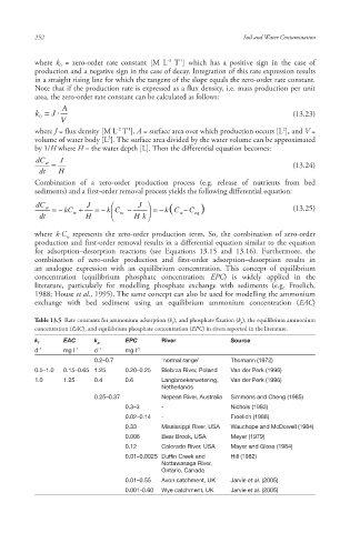
Table 13.5 Rate constants for ammonium adsorption (k f ), and phosphate fixation (k p ), the equilibrium ammonium
concentration (EAC), and equilibrium phosphate concentration (EPC) in rivers reported in the literature.
EAC EPC River Source
k f k p
d -1 mg l -1 d -1 mg l -1
0.2–0.7 ‘normal range’ Thomann (1972)
0.5–1.0 0.15–0.65 1.25 0.20–0.25 Biebrza River, Poland Van der Perk (1996)
1.0 1.25 0.4 0.6 Langbroekerwetering, Van der Perk (1996)
Netherlands
0.25–0.37 Nepean River, Australia Simmons and Cheng (1985)
0.3–3 - Nichols (1983)
0.02–0.14 - Froelich (1988)
0.33 Mississippi River, USA Wauchope and McDowell (1984)
0.006 Bear Brook, USA Meyer (1979)
0.12 Colorado River, USA Mayer and Gloss (1984)
0.01–0.0025 Duffin Creek and Hill (1982)
Nottawasaga River,
Ontario, Canada
0.01–0.55 Avon catchment, UK Jarvie et al. (2005)
0.001-0.60 Wye catchment, UK Jarvie et al. (2005)

10/1/2013 6:45:14 PM
Soil and Water.indd 264 10/1/2013 6:45:14 PM
Soil and Water.indd 264