Page 282 - Soil and water contamination, 2nd edition

15

Model calibration and validation

15.1 INTRODUCTION

In the previous chapters, a wide range of both physically based and empirical mathematical
equations has been presented that may be used to model the transport and fate of substances
in soil and water. The equations presented can be used alone, to tackle simple problems,
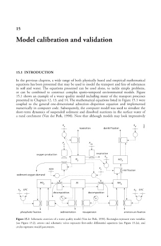
or can be combined to construct complex spatio-temporal environmental models. Figure
15.1 shows an example of a water quality model including many of the transport processes
presented in Chapters 12, 13, and 14. The mathematical equations listed in Figure 15.1 were
coupled to the general one-dimensional advection–dispersion equation and implemented
numerically in computer code. Subsequently, the computer model was used to simulate the
short-term dynamics of suspended sediment and dissolved nutrients in the surface water of
a rural catchment (Van der Perk, 1998). Note that although models may look impressively

k k
a d 6642 6642 6642
reaeration denitrification

F F
p res
respiration
oxygen production
k
O n NO
2 3
SOD k s
nitrification
sediment oxygen demand

PO SS NH
4 4
k EPC k EAC
P f
decomposition decomposition
F F
S R

phosphate fixation sedimentation resuspension ammonium fixation
Figure 15.1 Schematic overview of a water quality model (Van der Perk, 1998). Rectangles represent state variables
(see Figure 15.2), arrows and schematic valves represent first-order differential equations (see Figure 15.2a), and
circles represent model parameters.

10/1/2013 6:45:21 PM
Soil and Water.indd 281 10/1/2013 6:45:21 PM
Soil and Water.indd 281