Page 286 - Soil and water contamination, 2nd edition

Model calibration and validation 273

spills occur. So, in these circumstances, the model predictions will deviate from reality. Such
deviations are generally acceptable if their cause is evident and the spills reoccur infrequently.
On the other hand, the effects of increased toxin concentrations on the biochemical
transformation rates are of scientific interest and may be incorporated and verified in some
ecotoxicological models. This example demonstrates that it is unfeasible for a model to be
validated for all possible and less likely conditions. This stresses the need for the range of
environmental conditions for which the model has proven to be adequate to be explicitly
described. The only way to gain confidence in the model’s results and to understand its
limitations is to test the model repeatedly.
In this chapter, the procedure of calibration and validation of environmental models
will be further elaborated upon, with special reference to the criteria for an adequate
model. These criteria are, in principle, the same for both model calibration and validation.
Subsequently, some aspects of the model choice are discussed from the viewpoints of the
purpose of the model and the interdependence between model structure and uncertainty.

15.2 MODEL PERFORMANCE CRITERIA
In order to evaluate whether the model’s performance is satisfactory, some criteria for model
calibration and validation should be established a priori. How well the model should fit the
observed data depends on the nature of the observations and the desired use of the model.
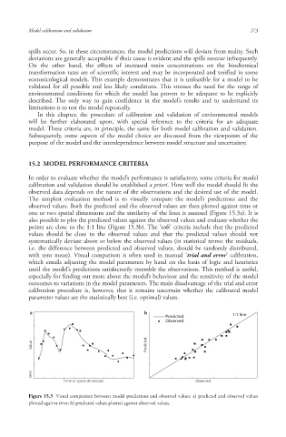
The simplest evaluation method is to visually compare the model’s predictions and the
observed values. Both the predicted and the observed values are then plotted against time or
one or two spatial dimensions and the similarity of the lines is assessed (Figure 15.3a). It is
also possible to plot the predicted values against the observed values and evaluate whether the
points are close to the 1:1 line (Figure 15.3b). The ‘soft’ criteria include that the predicted
values should be close to the observed values and that the predicted values should not
systematically deviate above or below the observed values (in statistical terms: the residuals,
i.e. the difference between predicted and observed values, should be randomly distributed,
with zero mean). Visual comparison is often used in manual ‘trial and error ’ calibration,
which entails adjusting the model parameters by hand on the basis of logic and heuristics
until the model’s predictions satisfactorily resemble the observations. This method is useful,
especially for finding out more about the model’s behaviour and the sensitivity of the model
outcomes to variations in the model parameters. The main disadvantage of the trial and error
calibration procedure is, however, that it remains uncertain whether the calibrated model
parameter values are the statistically best (i.e. optimal) values.

a b 1:1 line
Predicted
Observed

Value Predicted

6642 6642 6642
Time or space dimension Observed

Figure 15.3 Visual comparison between model predictions and observed values: a) predicted and observed values
plotted against time; b) predicted values plotted against observed values.

10/1/2013 6:45:21 PM
Soil and Water.indd 285
Soil and Water.indd 285 10/1/2013 6:45:21 PM